Thermal models

OghmaNano supports electro-thermal simulation in several levels of physical detail, ranging from a simple fixed-temperature approximation to fully coupled self-heating and (in exceptional regimes) hydrodynamic energy-balance transport. The purpose of these options is pragmatic: many device behaviours under bias cannot be explained using a purely electrical, fixed-temperature model once power dissipation becomes significant.

There are three options for thermal simulation in OghmaNano: (1) a constant temperature through the device (300 K by default); (2) a lattice thermal solver which solves the heat equation throughout the device including self-heating; and (3) a hydrodynamic (energy-balance) solver which does not assume the electron, hole, and lattice temperatures are equal. The constant-temperature option is recommended for most low-power simulations. The lattice thermal model is used when self-heating is expected to alter JV curves, recombination profiles, or device stability. The hydrodynamic model is intended for specialised cases such as strong heterojunction energy exchange or extreme fields where carriers may not relax to the lattice temperature locally.

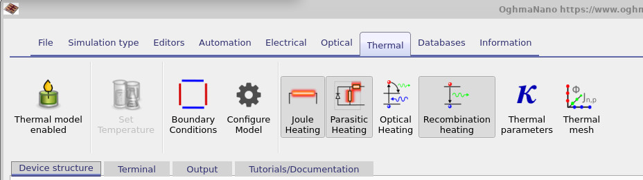
Thermal configuration is exposed through the Thermal ribbon, which provides access to: enabling/disabling the thermal model, selecting heat-generation terms (transport/Joule/Peltier, recombination, optical absorption, parasitic losses), setting thermal boundary conditions, choosing thermal mesh settings, and editing material thermal parameters. These controls are shown in ??.

How the electro-thermal solver is coupled

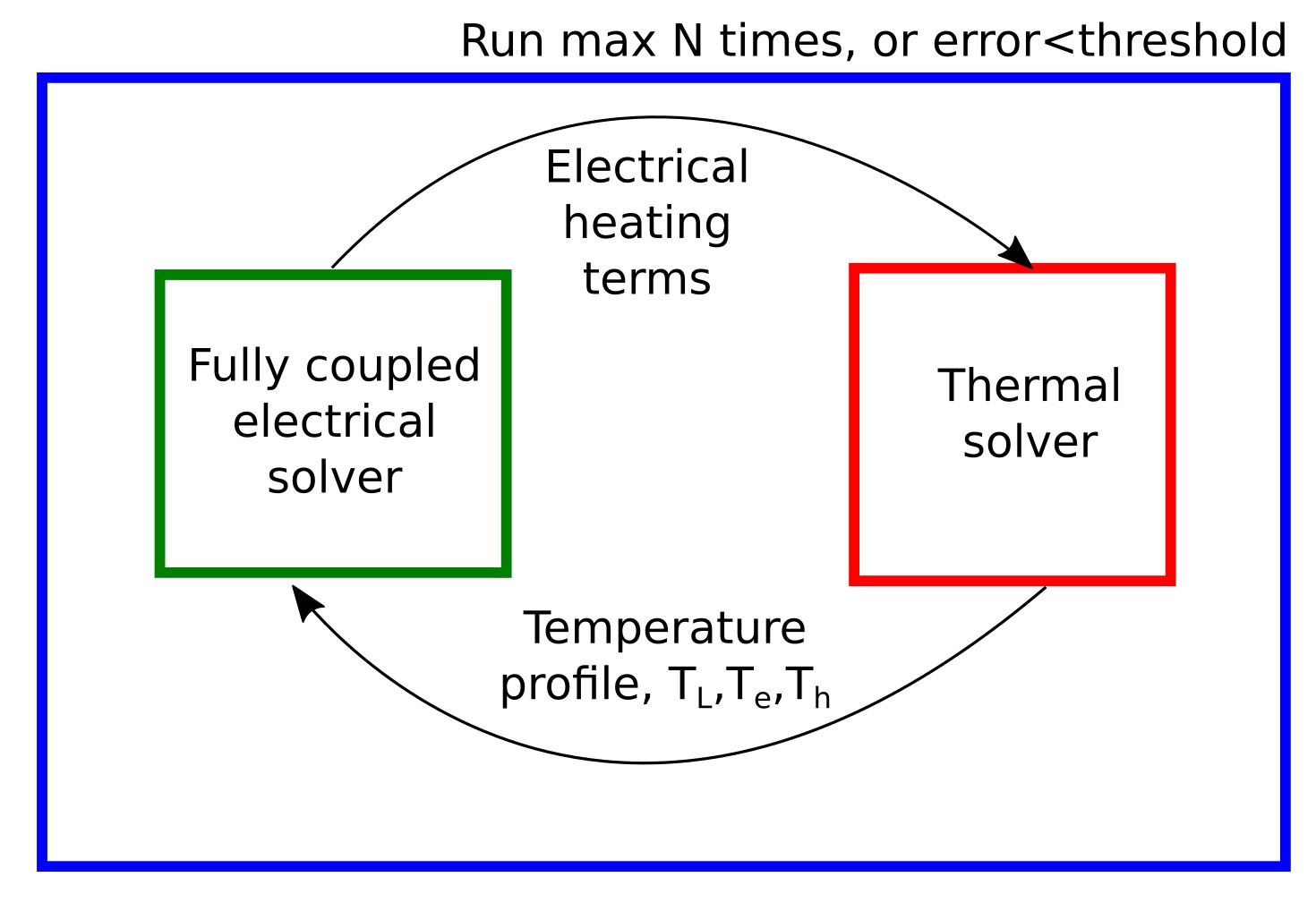
Electro-thermal simulation is inherently a coupled multi-physics problem. The electrical solution determines the spatial distribution of current, recombination, and power dissipation; those quantities become heat sources in the thermal diffusion equation; and the resulting temperature field feeds back into transport, recombination, and material properties. In OghmaNano this coupling is handled by an outer iteration loop: at a given bias point, the electrical solver runs using the current estimate of temperature, heat-generation terms are evaluated, the thermal solver updates the temperature field, and the process repeats until both the electrical residuals and thermal residuals meet convergence criteria.

This is the practical reason electro-thermal runs are slower than fixed-temperature runs: at each voltage step the electrical Newton solve may be executed multiple times, interleaved with thermal solves, until the joint solution stabilises. The aim is not “a temperature plot”; the aim is a self-consistent JV and internal state where dissipation and heat extraction are balanced.

Why thermal and electrical problems live on different length scales

A key structural feature of electro-thermal modelling is the mismatch of physical length scales. Electrical transport in thin-film devices is typically dominated by nanometre-to-micrometre structures: active layers, junction regions, injection zones, and narrow recombination profiles. Thermal diffusion, by contrast, depends on the entire heat-flow pathway: contacts, substrates, encapsulants, mounts, and sinks that are often millimetres to centimetres in scale. Attempting to mesh a centimetre-scale heatsink at thin-film electrical resolution is computationally pointless.

This is why OghmaNano treats thermal configuration as a first-class modelling object rather than an afterthought: the thermal problem is not just “more physics”, it is often a different domain. The thermal mesh can extend beyond the electrically active region, and boundary conditions are used to represent effective heat extraction without explicitly meshing macroscopic sinks.

Boundary conditions largely determine how hot the device gets

Thermal boundary conditions do not merely tidy up the mathematics: they define the heat escape route. A device with poor heat extraction can reach high temperatures rapidly once power dissipation increases; a device clamped to an effective sink can remain close to ambient even under significant current. In steady-state, the temperature rise is set by the balance “generated heat” versus “removed heat”, and boundary conditions largely specify the latter.

A useful physical analogy is a bath. The tap corresponds to heat generation; the plughole corresponds to heat extraction. If the plughole is open, water level stays low. If it is partially blocked, the water level rises. If it is blocked and the tap runs, the bath overflows. In the thermal problem the “water level” corresponds to the temperature field: if heat cannot leave effectively, temperature rises until the thermal gradients and boundary flux can carry away the generated power.

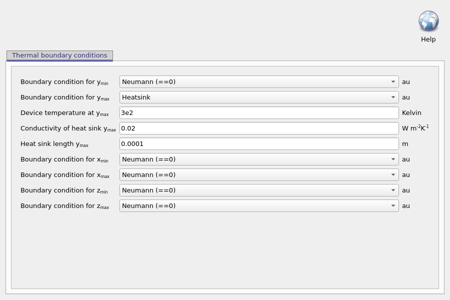
In the boundary-condition editor, “Neumann (==0)” corresponds to a zero normal heat flux boundary:

\[ -k \nabla T \cdot \hat{n} = 0 \]

Physically, this is an insulating face: the solver is instructed that heat does not flow through that surface. This does not imply the device is thermally isolated overall; it implies that particular face is not part of the intended heat-removal pathway. Heat extraction is then provided via the boundary (or boundaries) configured as heatsinks or other heat-transfer conditions.

Thermal parameters: conductivity and carrier energy relaxation times

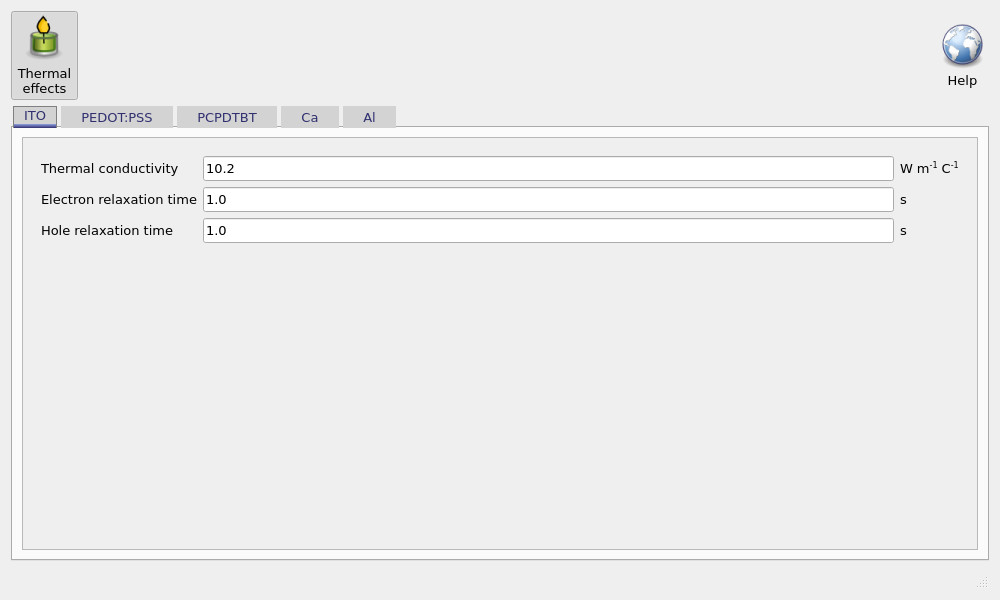
In addition to boundary conditions, the other dominant input to any thermal prediction is the set of thermal material parameters, particularly thermal conductivity. These are edited per layer via the Thermal parameters control (often shown as \(k\) or \(\kappa\)) in the Thermal ribbon (??), which opens the thermal-parameter editor shown in ??.

The key parameter is the thermal conductivity, which determines how readily heat diffuses through each layer and therefore how strongly temperature gradients build up under bias. The editor also exposes electron relaxation time and hole relaxation time. These relaxation-time parameters are only required when using the hydrodynamic (energy-balance) model, where carriers can have temperatures different from the lattice. In the standard lattice thermal model they are not used.

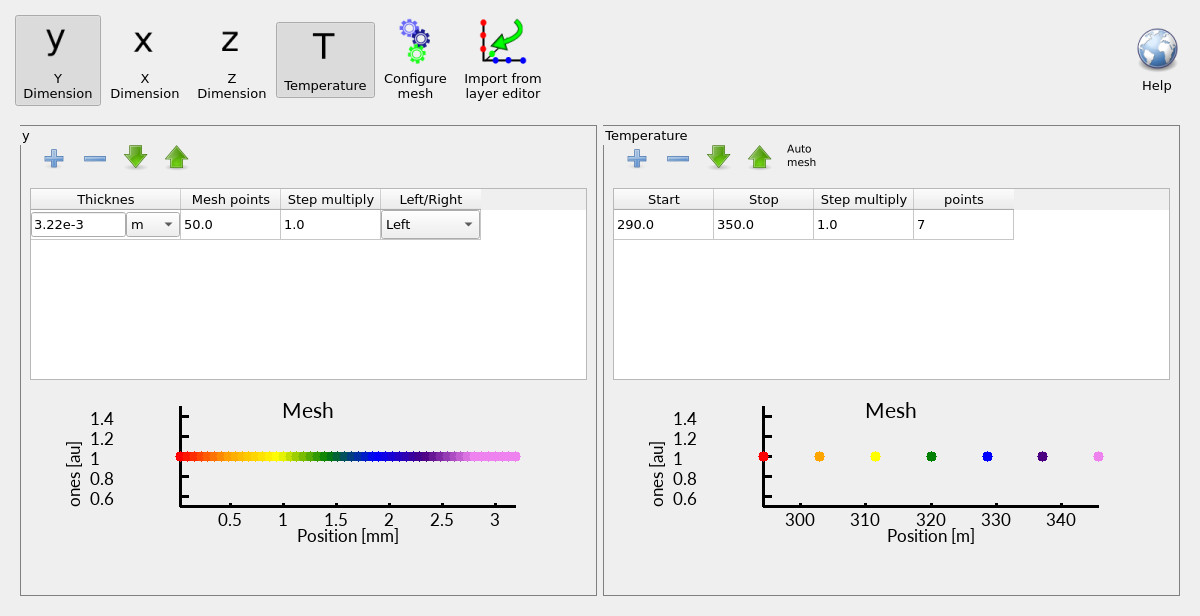
Temperature discretisation and precomputed tables

The thermal mesh configuration also includes a temperature range and a number of temperature points. These are not spatial mesh points; they form a discrete temperature grid used for precomputed temperature-dependent tables. Many internal model quantities are expensive to evaluate repeatedly as functions of temperature (and often quasi-Fermi level), so OghmaNano precomputes them on a finite temperature grid and interpolates during the coupled solve. This improves stability and reduces the computational cost of repeatedly evaluating temperature-dependent statistics inside the electro-thermal coupling loop.

Practically, this means the temperature range should comfortably bracket the temperatures expected during simulation. If a device self-heats beyond the configured range, interpolation may become extrapolation or clamping (depending on configuration), which is not desirable for quantitative self-heating analysis.

Multiple temperatures: lattice, electrons, and holes

It is also important to recognise that electro-thermal modelling naturally involves multiple temperatures. OghmaNano distinguishes the lattice temperature \(T_L\), an electron temperature \(T_e\), and a hole temperature \(T_h\). In the standard lattice thermal model, \(T_e\) and \(T_h\) are assumed to be equal to \(T_L\) (carriers are locally thermalised). In the hydrodynamic energy-balance model, \(T_e\) and \(T_h\) may deviate from \(T_L\), reflecting non-equilibrium carrier energy transport.

The hydrodynamic option is therefore not “a more accurate default”; it is a model for exceptional regimes where local carrier thermalisation is not a good approximation. For most thin-film and organic device simulations, the lattice thermal model captures the dominant thermal feedback at a reasonable computational cost.

Lattice thermal model

When solving only the lattice heat equation heat transfer and generation is given by

\[0 = \nabla \kappa_{l} \nabla T_{L} +H_j +H_r +H_{optical}+H_{shunt}\]

where joule heating (\(H_j\)) is give by

\[H_j= J_{n} \frac{\nabla E_{c}}{q} + J_{h} \frac{\nabla E_{h}}{q} ,\]

In practice, this transport-related heating term can include both conventional resistive (Joule) heating and interfacial Peltier heating/cooling when band edges vary strongly in space. The sign and localisation of this term can therefore carry physical information about where energy is being deposited into (or extracted from) the lattice by carrier transport.

recombination heating (\(H_r\)) is given by,

\[H_r=R(E_{c}-E_{v})\]

optical absorption heating is given by,

\[H_{optical}\]

and heating due to the shunt resistance is given by

\[H_{shunt}=\frac{J_{shunt} V_{applied}}{d}.\]

The thickness of the device is given by d. Note shunt heating is only in there to conserve energy conservation. In practice, parasitic series/shunt dissipation is often not spatially localised in a known microscopic way, so it is treated as an effective heat contribution required to close the energy balance of the simulated device.

Energy balance - hydrodynamic transport model

If you turn on the electrical and hole thermal model, then the heat source term will be replaced by

\[H=\frac{3 k_{b}}{2} \Bigg ( n (\frac{T_{n}-T_{l}}{\tau_{e}}) + p (\frac{T_{p}-T_{l}}{\tau_{h}})\Bigg) +R(E_{c}-E_{v})\]

and the energy transport equation for electrons

\[S_n=-\kappa_n \frac{dT_{n}}{dx}-\frac{5}{2} \frac{k_{b}T_{n}}{q} J_{n}\]

and holes,

\[S_p=-\kappa_p \frac{dT_{p}}{dx}+\frac{5}{2} \frac{k_{b}T_{p}}{q} J_{p}\]

will be solved.

The energy balance equations will also be solved for electrons,

\[\frac{dS_{n}}{dx}=\frac{1}{q}\frac{dE_{c}}{dx} J_{n}-\frac{3 k_{b}}{2} \Bigg( R T_{n}+ n(\frac{T_{n}-T_{l}}{\tau_{e}}) \Bigg)\]

and for holes

\[\frac{dS_{p}}{dx}=\frac{1}{q}\frac{dE_{v}}{dx} J_{p}-\frac{3 k_{b}}{2} \Bigg( R T_{p}+ n(\frac{T_{p}-T_{l}}{\tau_{e}}) \Bigg)\]

The thermal conductivity of the electron gas is given by

\[\kappa_{n}=\Bigg ( \frac{5}{2} +c_n\Bigg) \frac{{k_{b}}^2}{q} T_{n} \mu_n n\]

and for holes as,

\[\kappa_{p}=\Bigg ( \frac{5}{2} +c_p\Bigg) \frac{{k_{b}}^2}{q} T_{p} \mu_p p\]

This hydrodynamic framework introduces explicit carrier energy fluxes and carrier-lattice relaxation via \(\tau_e\) and \(\tau_h\). It is therefore substantially more expensive than the lattice thermal model and should be used only when the physics demands it. For most electro-thermal device studies, the lattice heat equation with well-chosen boundary conditions and layer conductivities captures the dominant self-heating feedback loop.

Full current expressions under non-isothermal conditions

The full thermally dependent drift diffusion transport equations as derived from the BTE are given by

\[\label{eq:Jnfull} \textbf{J}_n = \mu_e n \nabla E_c +\frac{2}{3} \mu_e n \nabla \bar{W} + \frac{2}{3} \bar{W} \mu_e \nabla n - \mu_e n \bar{W} \frac{\nabla m^*_e}{m^*_e}\]

\[\label{eq:Jpfull} \textbf{J}_p = \mu_h p \nabla E_v -\frac{2}{3} \mu_h p \nabla \bar{W} - \frac{2}{3} \bar{W} \mu_h \nabla p + \mu_p p \bar{W} \frac{\nabla m^*_h}{m^*_h}\]

where \(\bar{W}\) is the average kinetic energy of the free carriers. If the average energy is assumed to be \(3/2kT\), these expressions return to the standard drift–diffusion equations. Note the full form of these equations is required when not using MB statistics.