Exciton Domain Tutorial (Part A): Run a 3D Exciton Domain Simulation
1. Introduction
Understanding how excitons are generated, transported, and dissociated is central to the operation of bulk heterojunction (BHJ) organic solar cells. In these systems, light is absorbed predominantly in the donor phase, generating bound electron–hole pairs known as excitons. These excitons must diffuse through the donor material and reach a donor–acceptor interface before decaying. At the interface they may dissociate into free electrons and holes, with a probability determined by the local morphology, dimensionality, and the relevant kinetic rate constants.
The balance between exciton diffusion, interfacial dissociation, and competing loss processes therefore plays a decisive role in setting the effective photogeneration efficiency. However, explicit exciton modelling has historically been avoided not because of conceptual difficulty, but because of parameter uncertainty. Exciton diffusion lengths, lifetimes, interfacial dissociation rates, radiative and non-radiative decay channels, and annihilation processes were often poorly constrained for a given material system. In many practical modelling workflows these effects were therefore absorbed into a single scalar photon efficiency factor, \(\eta_{\mathrm{photon}}\), representing net geminate losses without resolving the underlying transport and kinetics.
This situation is now changing. Advances in experimental characterisation are beginning to provide direct measurements of exciton lifetimes, diffusion lengths, and loss channels in BHJ-like systems. As these parameters become better constrained, explicit exciton-domain modelling becomes increasingly informative—not as a means of predicting absolute device efficiencies, but as a way to explore how domain size, dimensionality, and material kinetics jointly determine an effective charge-generation yield. The exciton-domain model used in this tutorial was developed and published as part of this recent experimental–modelling work (see, for example, Nature Materials 21, 55–61 (2022)).
In this tutorial we therefore adopt an idealised but fully three-dimensional unit-cell geometry: a donor domain embedded within an acceptor matrix, represented initially as a donor sphere inside an acceptor box. While the geometry is simplified, the model treats exciton generation, diffusion, interfacial dissociation, and competing loss processes explicitly. This makes it a practical and physically transparent framework for exploring how experimentally measured parameters interact, for checking their internal consistency, and for developing intuition about how morphology and kinetics together control the effective photogeneration efficiency in three dimensions.
2. Governing equations
In this tutorial, exciton transport is treated explicitly by solving the three-dimensional exciton diffusion equation throughout the simulation domain. When the exciton model is enabled, optical absorption feeds directly into the exciton population, which then evolves according to the following equation:
\[ \frac{\partial X}{\partial t} = \nabla \cdot \left( D \nabla X \right) + G_{\mathrm{optical}} - k_{\mathrm{dis}} X - k_{\mathrm{FRET}} X - k_{\mathrm{PL}} X - \alpha X^2. \]
Here \(X(\mathbf{r},t)\) is the exciton density (\(\mathrm{m^{-3}}\)) and \(D\) is the exciton diffusion coefficient (\(\mathrm{m^2\,s^{-1}}\)). The source term \(G_{\mathrm{optical}}\) (\(\mathrm{m^{-3}\,s^{-1}}\)) represents exciton generation due to optical absorption. The remaining terms describe the competing processes that remove excitons from the population:
- Dissociation (\(k_{\mathrm{dis}} X\)): conversion of excitons into free electrons and holes at donor–acceptor interfaces. This is the productive channel that ultimately contributes to charge generation.
- Förster-type transfer (\(k_{\mathrm{FRET}} X\)): non-radiative energy transfer of excitons to neighbouring sites or domains, which redistributes exciton energy without directly generating free carriers.
- Radiative loss (\(k_{\mathrm{PL}} X\)): recombination of excitons via photon emission (photoluminescence), representing an intrinsic loss pathway.
- Annihilation (\(\alpha X^2\)): bimolecular exciton–exciton annihilation at high densities, which becomes important under strong excitation or in confined geometries.
The diffusion coefficient \(D\) is parameterised using an exciton diffusion length \(L\) (m) and exciton lifetime \(\tau\) (s) via
\[ D = \frac{L^2}{\tau}. \]
In this tutorial we run an exciton-only simulation: the solver computes the three-dimensional exciton density \(X(\mathbf{r})\) and the associated reaction terms, but it does not solve electron and hole transport. The dissociation term \(k_{\mathrm{dis}} X\) is therefore interpreted as a spatially resolved potential charge-generation rate, indicating where and how efficiently excitons would convert into free carriers at donor–acceptor interfaces.
3. Create the exciton-domain simulation
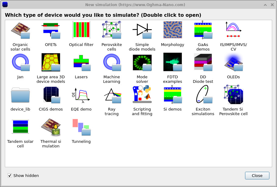
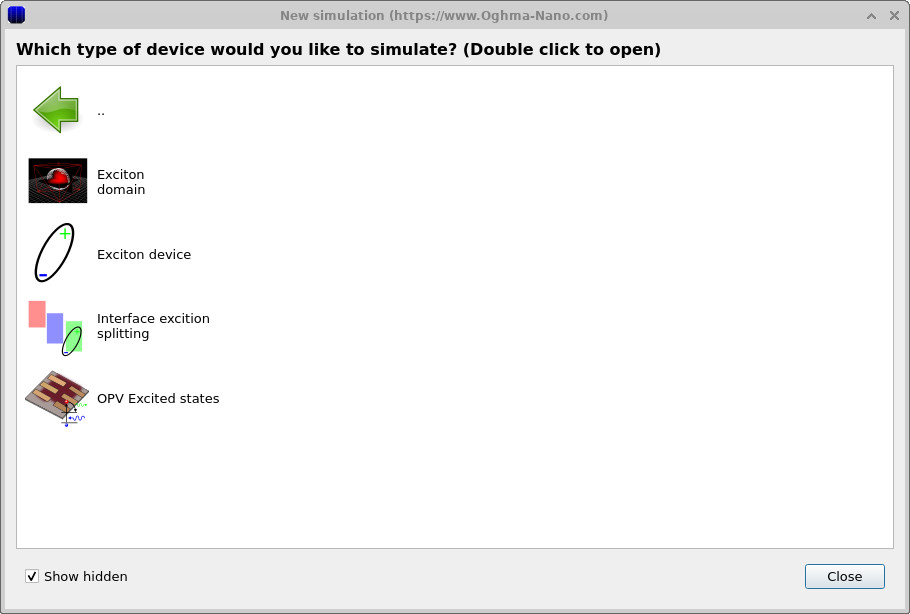
Open the New simulation window (Figure ??). This can be accessed by clicking New simulation in the main window. If you double-click on Exciton simulations, you will see the exciton library (Figure ??). Double-click Exciton domain to open the example project.
4. Inspect the geometry and parameters
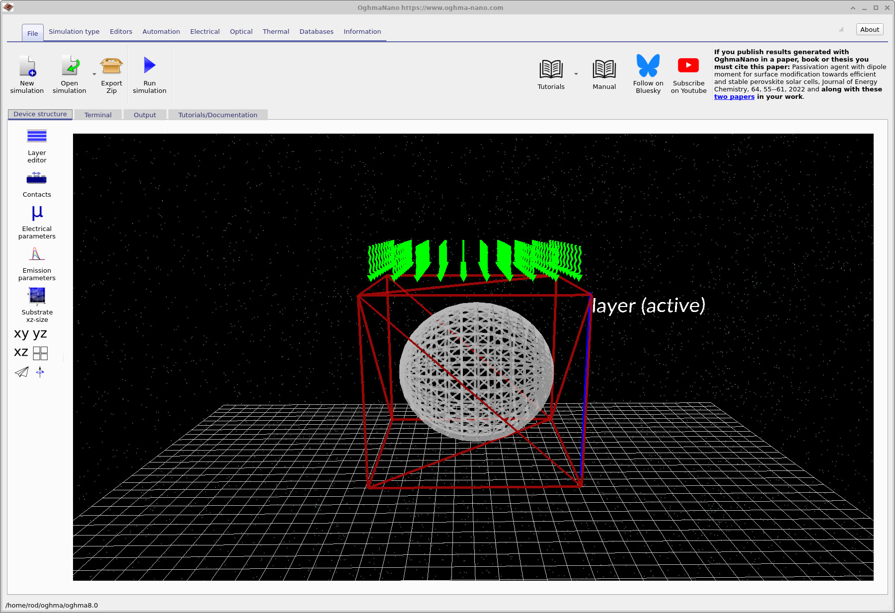
After opening the example, the main window displays a simple three-dimensional scene: a donor sphere embedded inside an acceptor box (Figure ??). The green rays indicate illumination incident from above. To inspect the exciton parameters, click Electrical parameters in the left-hand panel (within the Device structure tab). This opens the electrical parameter editor. If you scroll to the bottom of this window, you will find a section labelled Excitons, where the exciton-specific parameters are listed separately for each object in the scene (the surrounding layer and the embedded sphere), as shown in Figures ?? and ??.
The exciton section defines the parameters appearing in the diffusion–reaction equation. These include the exciton scattering length \(L\), which sets the diffusion coefficient via \(D = L^{2}/\tau\), and the exciton lifetime \(\tau\), which controls the overall timescale for transport in the absence of additional loss channels. Radiative recombination is described by the photoluminescence rate \(k_{\mathrm{PL}}\), while non-radiative energy transfer processes are captured by the Förster-type rate \(k_{\mathrm{FRET}}\). At higher exciton densities, bimolecular annihilation is included through the coefficient \(\alpha\), corresponding to the \(-\alpha X^{2}\) term in the governing equation. Finally, the dissociation rate \(k_{\mathrm{dis}}\) specifies how efficiently excitons convert into charge-transfer states at donor–acceptor interfaces and is the key parameter controlling the effective charge-generation efficiency in this model.
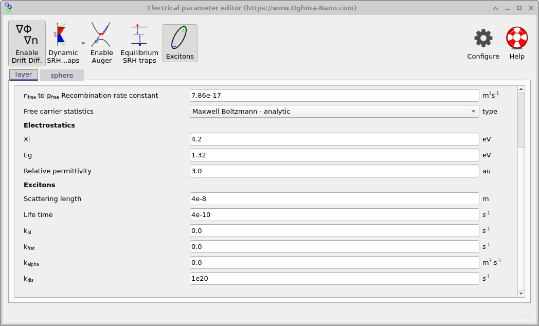
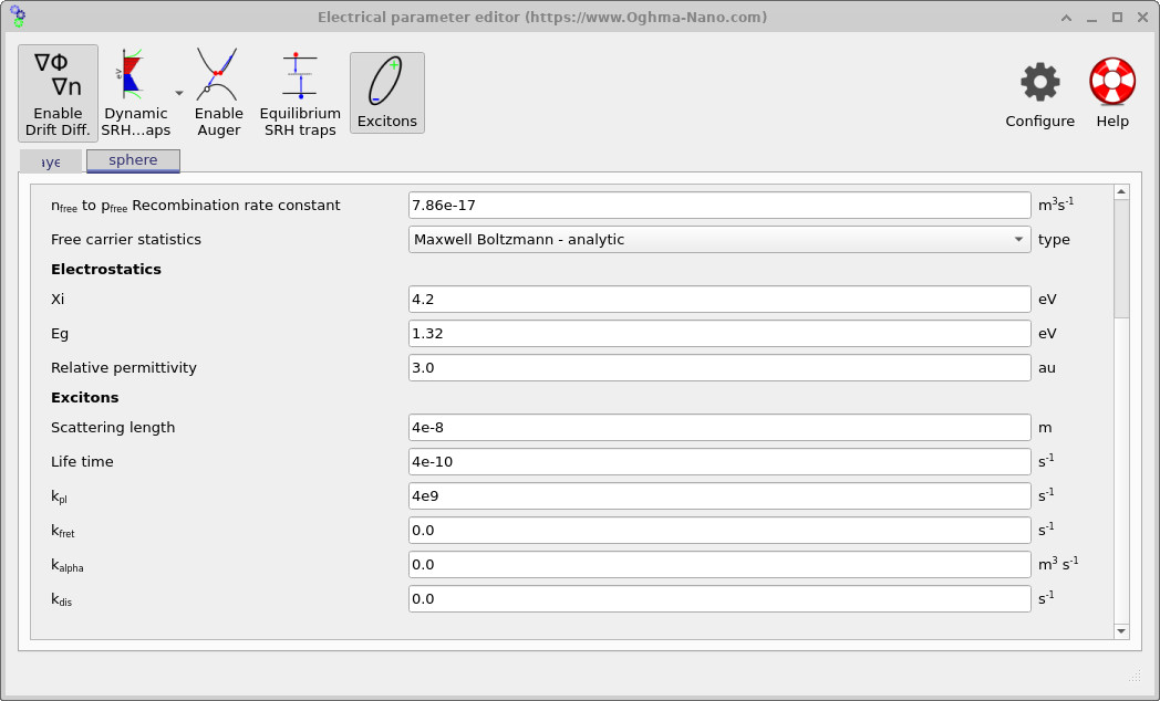
The key conceptual feature of this example is that the sphere (donor) and the layer (acceptor matrix) use different exciton physics. In the screenshots above, the donor sphere includes a non-zero \(k_{\mathrm{PL}}\) (a loss channel). The surrounding region is configured with a very large \(k_{\mathrm{dis}}\), so once excitons reach (or leave into) that region they dissociate quickly. That makes the donor/acceptor boundary behave like an efficient sink, producing the characteristic “high in the centre, depleted near the boundary” profile.
5. Run the simulation
Click the blue Run simulation triangle to start the solver. The terminal output
will appear in the main window, as shown in Figure
??.
The initial lines report general information about the simulation setup and geometry.
The key diagnostic appears once the exciton solver starts running and has the form
Exciton f() = … , steps = …. This line reports the progress of the three-dimensional exciton solver.
The quantity f() is a residual measuring how far the current exciton density field
is from self-consistency; as the solver iterates, this value should decrease.
The accompanying steps counter indicates the iteration number.
In the example shown, the residual drops from an initial value to
2.97 × 10⁴ by step 2, after which the solver reports
that the equation has been solved and terminates.
On a typical modern laptop, this example should complete in around 5–10 seconds. If the run time extends to minutes, this usually indicates that the mesh is excessively fine or that the geometry or parameters have been modified in a way that greatly increases the number of mesh points. In that case, it is worth revisiting the mesh settings or retracing the previous setup steps before proceeding.
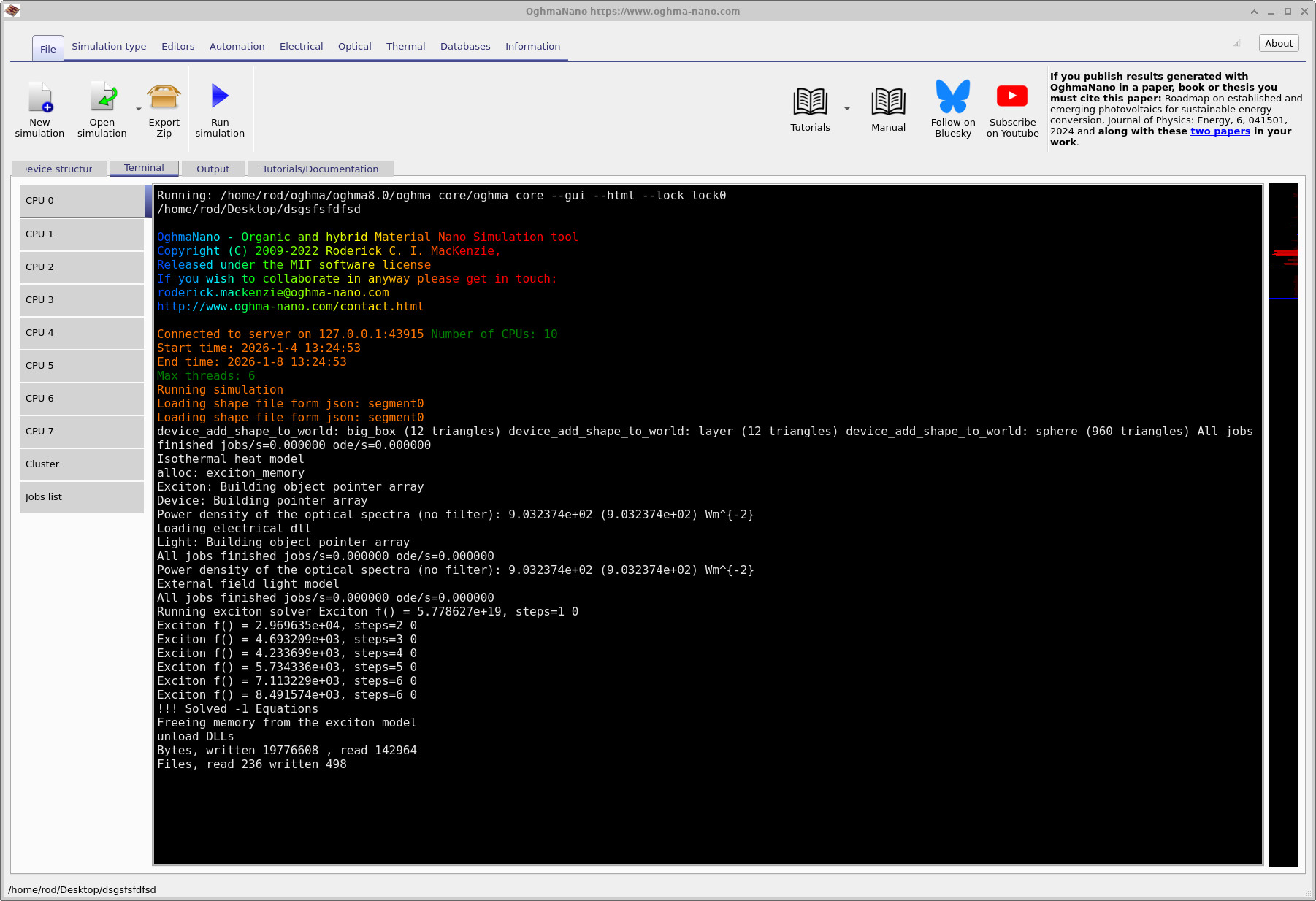
Exciton f() decreases as the solver converges.
exciton_output/.
exciton_output/. The files are plain CSV and can be opened
in OghmaNano’s viewers or external tools.
6. Plotting the output
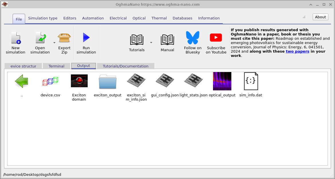
Once the run has finished, switch to the Output tab (Figure
??).
The most relevant items for this tutorial are the exciton_output/ directory,
which contains the spatially resolved exciton results, and the file
exciton_sim_info.json, which summarises global generation and loss statistics
and will be used later in Part C.
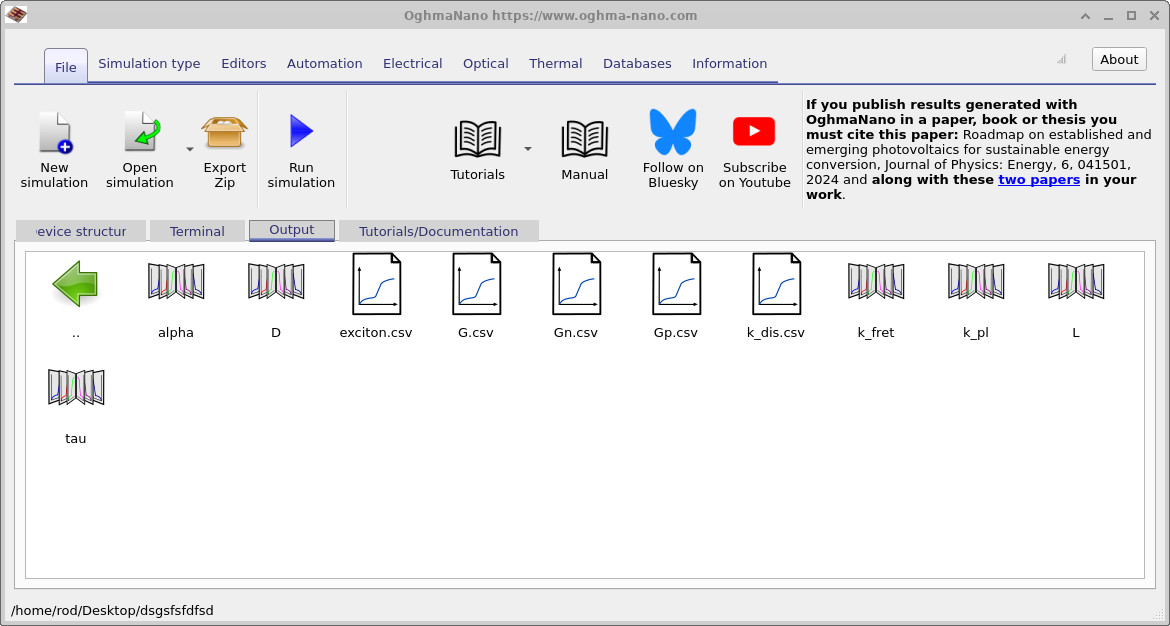
Double-clicking exciton_output/ reveals the contents shown in Figure
??.
Open G.csv to view the exciton generation rate produced by the optical model (Figure
??).
In the 3D plot window you can rotate the scene with the mouse and use the
Z and Y sliders at the bottom to slice through the volume.
This is often the fastest way to verify that the geometry, illumination direction, and mesh
are behaving as intended.
Next, open exciton.csv (Figure
??),
which shows the steady-state exciton density.
You should observe the characteristic signature of diffusion to an interfacial sink:
a high exciton density in the interior of the donor sphere, with depletion toward the
donor–acceptor boundary where dissociation is strong.
Use the slicing sliders to confirm that this depletion follows the interface geometry
rather than being an artefact of the viewing angle.
Finally, open Gn.csv (Figure
??),
which shows the spatially resolved electron generation rate arising from exciton
dissociation.
In this example you should see a distinctive ring (or shell) of generation
localised near the donor–acceptor interface.
Use the Z and Y sliders to move the slicing plane through the
volume and explore how this dissociation profile evolves with position.
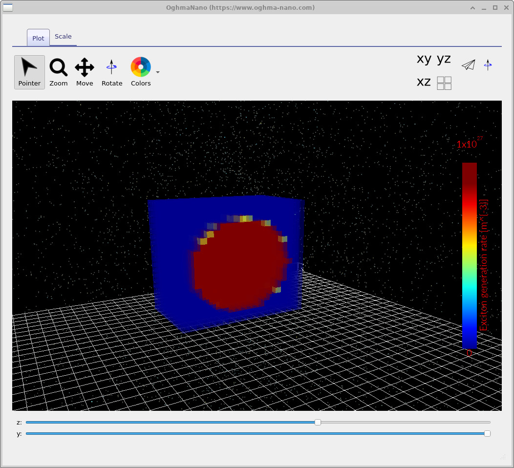
G.csv: exciton generation rate \(G_{\mathrm{optical}}\) from the optical model (units \(\mathrm{m^{-3}\,s^{-1}}\)).
Rotate and slice (Z/Y sliders) to inspect spatial localisation.
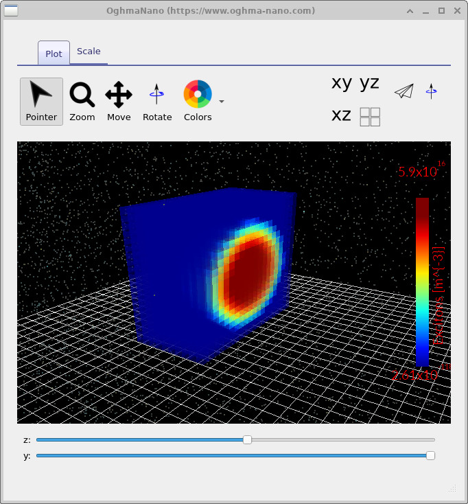
exciton.csv: exciton density \(X\) (units \(\mathrm{m^{-3}}\)).
The “centre-high / boundary-low” profile is the expected outcome of diffusion toward a fast-dissociation sink.
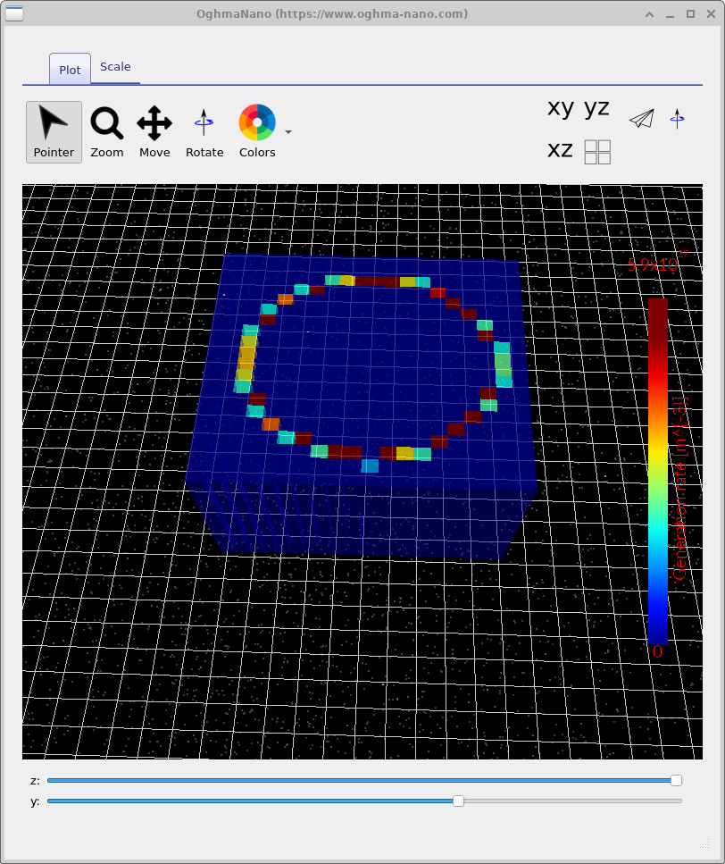
Gn.csv: electron generation rate from exciton dissociation (units \(\mathrm{m^{-3}\,s^{-1}}\)).
Dissociation is concentrated at the donor/acceptor interface, producing a characteristic ring/shell in slices.
Use the Z/Y sliders to explore how this feature changes with position.
7. What are the files in exciton_output/?
The exciton_output/ directory contains two distinct types of files.
The first group consists of computed fields produced by the exciton solver,
such as the exciton density and dissociation-derived generation rates.
The second group contains parameter maps: three-dimensional copies of the
exciton parameters defined in the GUI. These are written out primarily as a
consistency and debugging aid, allowing you to verify that the intended material
parameters have been applied correctly in space. Tables 1 and 2 summarise these two categories. All quantities are reported in SI units.
(Some files may not be written if the corresponding sub-models are disabled.)
| File name | Description | Typical units |
|---|---|---|
exciton.csv |
Exciton density field \(X(\mathbf{r})\) | \(\mathrm{m^{-3}}\) |
G.csv |
Exciton generation rate \(G_{\mathrm{optical}}(\mathbf{r})\) | \(\mathrm{m^{-3}\,s^{-1}}\) |
Gn.csv |
Electron generation rate from exciton dissociation | \(\mathrm{m^{-3}\,s^{-1}}\) |
Gp.csv |
Hole generation rate from exciton dissociation | \(\mathrm{m^{-3}\,s^{-1}}\) |
D |
Exciton diffusion coefficient \(D\) | \(\mathrm{m^{2}\,s^{-1}}\) |
alpha |
Exciton–exciton annihilation contribution \(\alpha X^2\) | \(\mathrm{m^{3}\,s^{-1}}\) |
| File name | Description | Typical units |
|---|---|---|
k_dis.csv |
Dissociation rate \(k_{\mathrm{dis}}(\mathbf{r})\) | \(\mathrm{s^{-1}}\) |
k_fret |
Förster-type transfer rate \(k_{\mathrm{FRET}}(\mathbf{r})\) | \(\mathrm{s^{-1}}\) |
k_pl |
Radiative (photoluminescent) loss rate \(k_{\mathrm{PL}}(\mathbf{r})\) | \(\mathrm{s^{-1}}\) |
L |
Exciton diffusion (scattering) length \(L(\mathbf{r})\) | \(\mathrm{m}\) |
tau |
Exciton lifetime \(\tau(\mathbf{r})\) | \(\mathrm{s}\) |
The parameter-map files in Table 2 are not solver outputs in the usual sense. They simply reflect the exciton parameters defined in the Electrical → Excitons section of the GUI, written out on the same three-dimensional mesh as the solution fields. Their purpose is to provide a transparent way to check that parameters are assigned to the correct objects and regions of the domain, particularly when working with complex geometries.
8.1 Interpreting exciton_sim_info.json (dissociation efficiency)
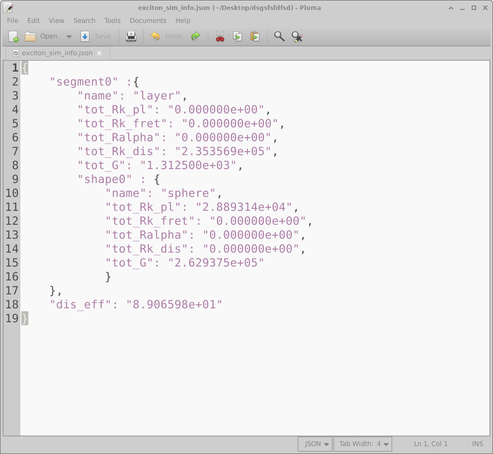
exciton_sim_info.json summary file, reporting spatially integrated
generation and loss channels for each object and the overall dissociation efficiency.
While the three-dimensional plots are invaluable for visualising where excitons are
generated, lost, and dissociated, they do not by themselves provide concise numerical summaries.
The file exciton_sim_info.json fills this role by reporting spatially integrated
generation and loss rates for each object in the simulation (the surrounding layer, the
embedded sphere, and any additional shapes you may add).
To view this information, open the main Output tab and double-click
exciton_sim_info.json. The file contains a nested JSON structure that lists, for each
object, the total exciton generation rate and the total rates associated with each competing
loss or dissociation channel. These quantities allow you to quantify how changes in material
parameters, geometry, or morphology translate into changes in charge-generation efficiency.
💡 Units: The quantities reported in this file are volume-integrated totals. Locally, generation and reaction rates are fields with units such as \(\mathrm{m^{-3}\,s^{-1}}\) (or \(\mathrm{m^{-3}}\) for densities). After integration over volume, the corresponding totals have units of \(\mathrm{s^{-1}}\), representing events per second.
The top-level key segment0 simply marks the start of the report.
Within it, the field name identifies the enclosing object (here, the
layer), while the nested shape0 block corresponds to the embedded
object (the sphere). Each block reports the total contribution of that object
to generation, dissociation, and loss processes.
Table 2 summarises the fields you will encounter in this file and how to interpret them.
| JSON field | Meaning | Typical units | Where it appears |
|---|---|---|---|
segment0 |
Container node for the report (not a physical quantity) | — | Top level |
name |
Object name (layer or embedded shape) | — | Inside segment0 and shape0 |
tot_G |
Total exciton generation rate, integrated over the object volume | \(\mathrm{s^{-1}}\) | Layer and shape blocks |
tot_Rk_pl |
Total radiative (photoluminescent) loss rate | \(\mathrm{s^{-1}}\) | Layer and shape blocks |
tot_Rk_fret |
Total Förster-type transfer loss or interaction rate | \(\mathrm{s^{-1}}\) | Layer and shape blocks |
tot_Ralpha |
Total exciton–exciton annihilation loss rate | \(\mathrm{s^{-1}}\) | Layer and shape blocks |
tot_Rk_dis |
Total exciton dissociation rate to free carriers | \(\mathrm{s^{-1}}\) | Layer and shape blocks |
dis_eff |
Overall dissociation efficiency (fraction of generated excitons that dissociate) | \(\%\) | Top level |
Taken together, the three-dimensional plots and the numerical summaries in
exciton_sim_info.json provide a complementary view of the simulation:
the plots show where processes occur, while the JSON file quantifies
how much each process contributes. This makes it a useful tool for
systematically analysing how changes in parameters or geometry affect exciton
dissociation and effective charge generation.
9. Putting it together
Taken together, the three-dimensional results tell a coherent physical story.
Optical absorption generates excitons primarily in the interior of the donor domain.
These excitons then diffuse through the donor, are depleted near the donor–acceptor interface,
and dissociate efficiently once they reach the surrounding acceptor region.
The spatial plots show where these processes occur; the summary report
exciton_sim_info.json quantifies how much each process contributes.
In this example, the summary report separates the underlying physics cleanly by spatial region, allowing generation, loss, and dissociation processes to be interpreted in a transparent way.
-
Sphere (donor):
Most optical absorption—and therefore most exciton generation—occurs inside the donor sphere,
reflected by a large value of
tot_Gin theshape0/sphereblock. Within the donor, the dominant competing loss channel in this example is radiative decay, quantified bytot_Rk_pl. The ratio oftot_Rk_pltotot_Gprovides a direct measure of how strongly radiative losses suppress the exciton population before it can reach the donor–acceptor interface. -
Layer (acceptor matrix):
The surrounding layer absorbs only weakly in this example, so its contribution to exciton
generation (
tot_G) is small. Its primary role is instead exciton conversion: the layer is configured with a strong dissociation channel, makingtot_Rk_disthe dominant term in thelayerblock. This corresponds directly to the interfacial dissociation observed in the spatial plots, whereGn.csvshows a ring- or shell-like region of electron generation concentrated at the donor–acceptor boundary.
The bottom-line metric dis_eff reports the overall dissociation efficiency
of the system (here approximately \(89\%\)).
Physically, this indicates that the majority of excitons generated in the donor diffuse to the
interface and dissociate, with only a relatively small fraction lost to radiative decay.
Other channels, such as Förster transfer or exciton–exciton annihilation, are inactive in this
particular example.
In other words, the simulation operates in a regime where interfacial dissociation outcompetes exciton decay, resulting in a high effective photon-to-free-carrier yield. This combination of three-dimensional visualisation and quantitative reporting provides a compact but physically complete picture of how geometry and kinetic parameters together determine charge-generation efficiency in an exciton-domain model.
👉 Next step: Continue to Part B, where we edit the domain geometry (sphere → arbitrary mesh) and adjust the optical generation settings to see how geometry and absorption interact with diffusion and dissociation.
📘 Return to the introduction to organic electronics for a broader overview of the topic.