Non-equilibrium carrier trapping and recombination using Shockley-Read-Hall trap states
1. Introduction
Many readers will first encounter Shockley–Read–Hall (SRH) recombination in their undergraduate physics classes. It is often introduced as a recombination mechanism between a free carrier and a trapped carrier, and is summarized by the following well-known and simplified expression:
\[R_{\mathrm{SRH}} = \frac{np - n_{i}^{2}} {\tau_{p}(n + n_{1}) + \tau_{n}(p + p_{1})} \]
where:
- \(\tau_{n}\), \(\tau_{p}\) are the electron and hole lifetimes associated with the trap,
- \(n_{1} = N_{C} \exp\!\big(-(E_{C} - E_{t})/k_{B}T\big)\) is the effective electron density when the trap lies in equilibrium,
- \(p_{1} = N_{V} \exp\!\big(-(E_{t} - E_{V})/k_{B}T\big)\) is the corresponding hole density,
- \(E_{t}\) is the trap energy level, and \(n_{i}\) is the intrinsic carrier concentration.
This equation was first derived in Shockley & Read, Physical Review 87, 835 (1952), and is described in more detail in the SRH theory section of the manual.
However, it is important to note that the equation above is not the full story. This compact form results from the original Shockley–Read–Hall analysis under a set of simplifying assumptions:
- Steady-state conditions: the trap occupancy is assumed not to vary in time, so capture and emission rates balance.
- Single trap level: recombination occurs through a single, energetically sharp defect level at energy \(E_t\) within the band gap.
These assumptions are perfectly adequate in materials with only a few impurities, where trap-assisted recombination plays only a minor role and a single discrete trap level provides a reasonable description. However, once Shockley–Read–Hall recombination becomes the dominant process, as is often the case in disordered semiconductors, the picture changes. In such systems, traps rarely occur at a single energy but instead form a broad distribution of states within the band gap, meaning that a density-of-states description is more appropriate. Moreover, the large number of occupied traps introduces substantial trapped charge, which acts not only as a recombination channel but also as a reservoir of carriers that reshapes the electrostatic potential across the device. This means the trap occupation must be treated self-consistently with Poisson’s equation rather than as a passive background process. In addition, the steady-state assumption prevents the description of dynamic processes: in time-resolved experiments or transient simulations the trap occupancy evolves in time, and this evolution itself is essential to the recombination dynamics. For these reasons, while the compact SRH formula is a valuable starting point, it must be generalized in materials with high trap densities or in situations where non-equilibrium dynamics are important.
To properly understand and account for these differences between the steady-state Shockley–Read–Hall formalism and the broader treatment given in the original work, we need to dig a little deeper into the underlying theory.
2. Understanding dynamic SRH rate equation
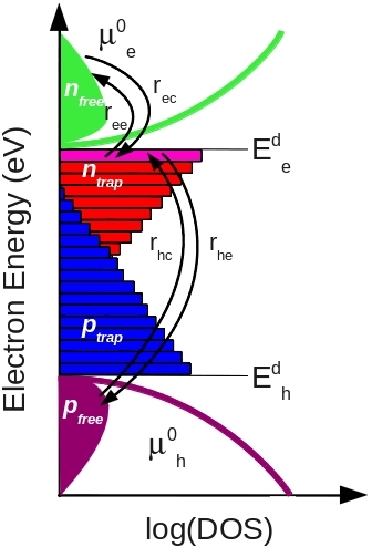
To really understand what the Shockley–Read–Hall (SRH) formalism means, we need to look carefully at the way the original authors set it up. What they did was to write a rate equation for the occupancy of a trap state within the semiconductor band gap. This rate equation is given below and is illustrated schematically in ??. It describes how the number of carriers in a trap changes due to capture and escape processes.
\[ \frac{dn_t}{dt} = r_{ec} - r_{ee} - r_{hc} + r_{he} \]
In this expression, the four terms correspond to the four possible carrier flows associated with an electron trap. The term \(r_{ec}\) represents electron capture from the free electron population into the trap, while \(r_{ee}\) represents electron emission back to the free band. Similarly, \(r_{hc}\) is the rate of hole capture into the trap, and \(r_{he}\) is the rate of hole emission back to the free hole population. Together these processes describe the detailed balance of carrier flow into and out of a single trap level.
It is useful to separate these contributions conceptually. The electron capture and emission terms (\(r_{ec}\), \(r_{ee}\)) describe pure charge trapping, as one would typically imagine for traps storing electrons. The hole capture and emission terms (\(r_{hc}\), \(r_{he}\)) describe recombination, since they represent the annihilation or recreation of trapped charge by interaction with the free hole population. The key point here is that the trap itself actually contains charge — it is not simply a mathematical sink for recombination, but a real reservoir of carriers that must be accounted for when modeling both recombination and the electrostatics of the device.
2. Escape v.s capture probability
The capture and escape rates for carriers interacting with a trap are summarized in the table below, while the corresponding escape probabilities are given in the equations below that. A key feature of Shockley–Read–Hall theory is the strong dependence of escape probability on the energetic depth of the trap. Carriers trapped close to a band edge can escape relatively easily, whereas carriers in deeper traps have a much lower probability of emission. This behavior is reflected directly in the exponential terms of the escape probability expressions. By contrast, the probability of a carrier being captured into a trap does not depend on trap depth; it depends only on whether the trap is empty or occupied. An empty trap is highly likely to capture an approaching carrier, while a fully occupied trap cannot capture additional carriers. Looking across Table 9.1, one can see these principles expressed mathematically in the capture and escape rates. Taken together, they describe a system in which carriers readily fall into traps, find it increasingly difficult to escape if the traps lie deeper in energy, and where both electrons and holes may be captured. Once both species occupy the same trap, recombination naturally occurs.
| Mechanism | Symbol | Expression |
|---|---|---|
| Electron capture rate | \(r_{ec}\) | \(n v_{th} \sigma_{n} N_{t} (1-f)\) |
| Electron escape rate | \(r_{ee}\) | \(e_{n} N_{t} f\) |
| Hole capture rate | \(r_{hc}\) | \(p v_{th} \sigma_{p} N_{t} f\) |
| Hole escape rate | \(r_{he}\) | \(e_{p} N_{t} (1-f)\) |
The escape probabilities are given by:
\[\label{eq:taile} e_n=v_{th}\sigma_{n} N_{c} exp \left ( \frac{E_t-E_c}{kT}\right )\]
and
\[ e_p = v_{th} \sigma_{p} N_{v} \exp\!\left( \frac{E_{v} - E_{t}}{kT} \right) \]
The occupation function is given by the equation, \[f(E_{t},F_{t})=\frac{1}{e^{\frac{E_{t}-F_{t}}{kT}}+1}\] Where, \(E_{t}\) is the trap level, and \(F_{t}\) is the Fermi-Level of the trap.
3. From one trap to a DoS
Up to this point, and as illustrated in Fig. 9.1, we have considered the behavior of a single trap level (the “purple trap”). In real disordered semiconductors, however, recombination is rarely dominated by one discrete state. Instead, there exists a distribution of trap levels that extends into the band gap from both the conduction and valence band edges. This means that we must describe not only electron traps but also hole traps, and their respective densities as a function of energy.
To do this, the trap density is described by a density-of-states function \(\rho(E)\), which can be set to any analytical form appropriate to the material under study. In this example, we use an exponential distribution of trap states:
\[ \rho^{e/h}(E) = N^{e/h} \exp\!\left( \frac{E}{E_{u}^{e/h}} \right), \]
where \(N^{e/h}\) is the density of states at the band edge (LUMO or HOMO) in units of states per eV, and \(E_{u}^{e/h}\) is the characteristic slope energy that defines the exponential tail. The effective trap density associated with a specific energy level is then obtained by averaging over the energy interval \(\Delta E\) that represents the trap:
\[ N_{t}(E) = \frac{ \int_{E - \Delta E / 2}^{E + \Delta E / 2} \rho^{e}(E)\, dE }{ \Delta E }. \]
In practice, the model discretizes the distribution into a finite number of trap levels. For each trap level we write a separate rate equation, as described earlier, and assign it a corresponding density \(N_t\). Typically, between three and twenty trap levels are used under both the conduction and valence bands, each of which can store charge. The total trapped charge is then coupled self-consistently to Poisson’s equation, ensuring that the electrostatic profile of the device accounts for the occupancy of traps.
Finally, the trap-assisted recombination terms appear explicitly in the carrier continuity equations. For example, the Shockley–Read–Hall recombination rate is written as
\[ R_{\mathrm{SRH}} = r_{hc} - r_{he} \;=\; r_{ec} - r_{ee}, \]
linking the capture and escape rates of electrons and holes directly to the balance of carriers in the conduction and valence bands. In this way, both trapping and recombination processes are described on equal footing, and their contributions are naturally integrated into the continuity and Poisson equations that govern device operation.
The final result
The outcome of solving the full set of Shockley–Read–Hall equations in both energy space and position space across the device is that we can describe where charge resides, not only in terms of position but also in terms of energy. This allows us to capture the charge dynamics that dominate in highly disordered materials. An example is shown in ??, where we simulate a J–V curve under dark conditions as the applied bias is increased from 0 V. As the bias rises, carriers are injected from the contacts and progressively fill the trap states. These trapped charges act simultaneously as recombination centers and as sources of space charge that reshape the electrostatic potential across the device. Without including these effects, any device simulation will be incomplete and likely incorrect. For a detailed discussion of why trap states must be included in such models, see this section.
👉 Next step: Now continue to Analytical steady state SRH recombination