Electrical Parameter editor

1. Introduction

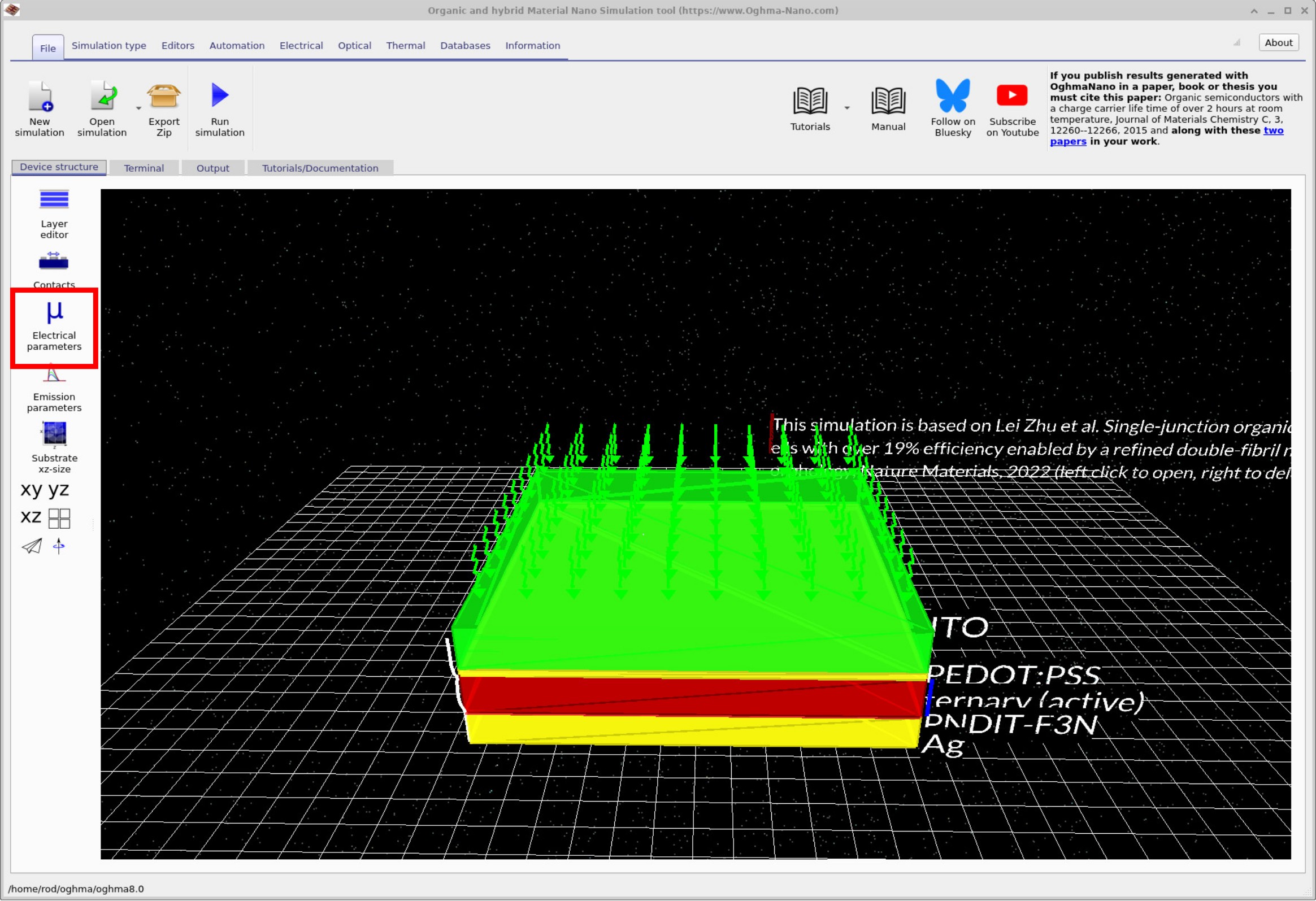
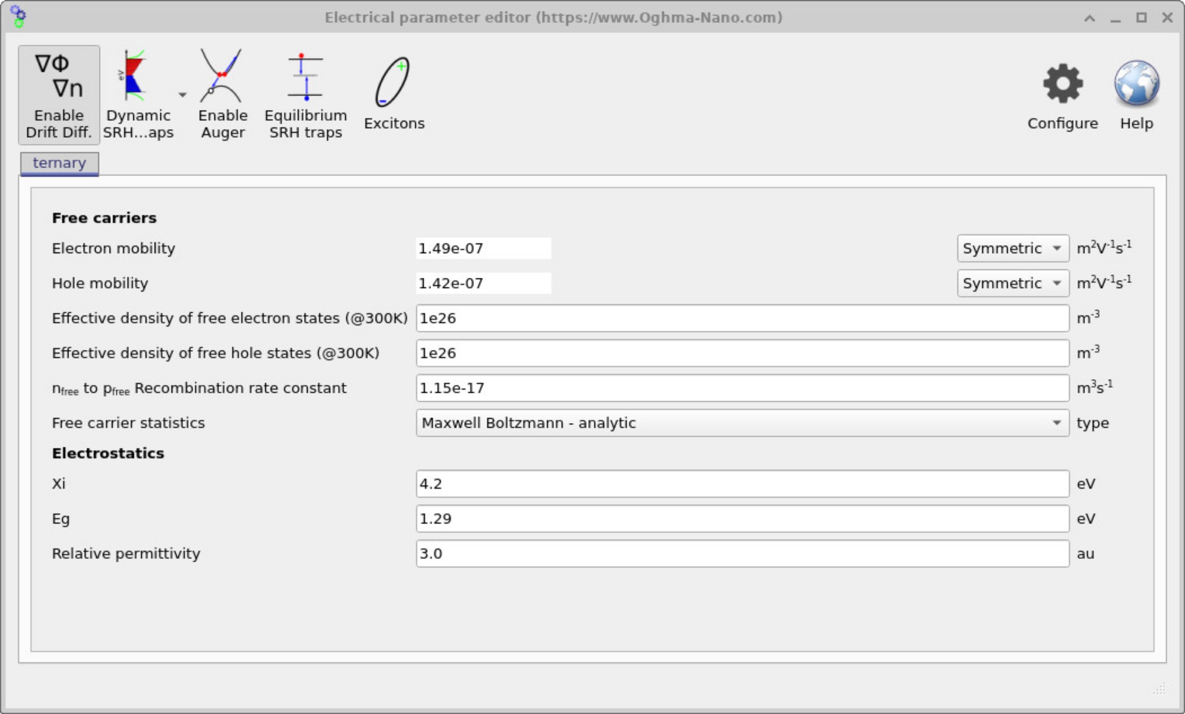
In OghmaNano, the Electrical parameter editor provides the interface for defining the transport and recombination properties of electrically active layers. To access it, click the Electrical parameters button in the Device structure tab of the main simulation window (see ??). When opened, the Electrical parameter editor displays a set of input fields where you can specify key quantities such as carrier mobilities, densities of states, recombination constants, and fundamental material properties like bandgap and permittivity (see ??). Importantly, only layers that have been marked as active in the Layer editor will appear in the Electrical parameter editor. If a layer is not set as active, its electrical properties cannot be edited, since drift–diffusion and recombination processes are not solved in those regions.

2. Basic electrostatics and drift–diffusion equations

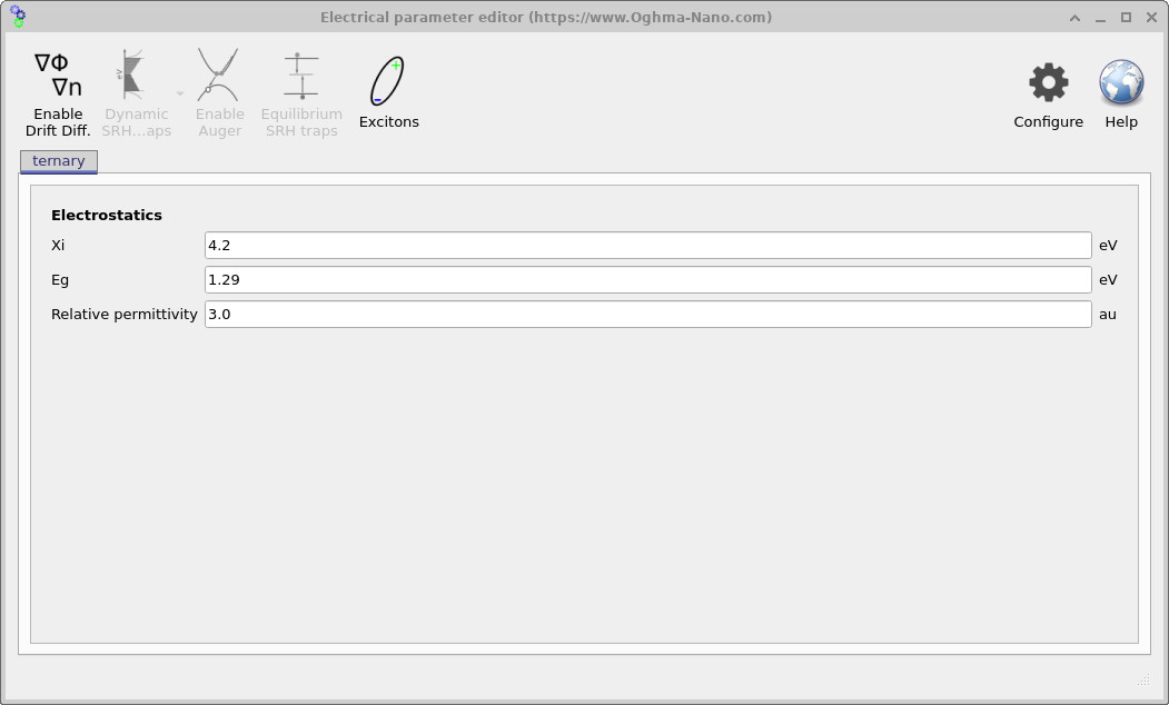
Figure ?? shows the Electrical parameter editor with no additional solver buttons activated. In this state, the drift–diffusion equations are disabled, but the Poisson equation is still solved. The interface therefore displays only the parameters needed for electrostatics: the electron affinity (χ), the band gap (E_g), and the relative permittivity (ε_r). These quantities define how the potential is distributed across the device.

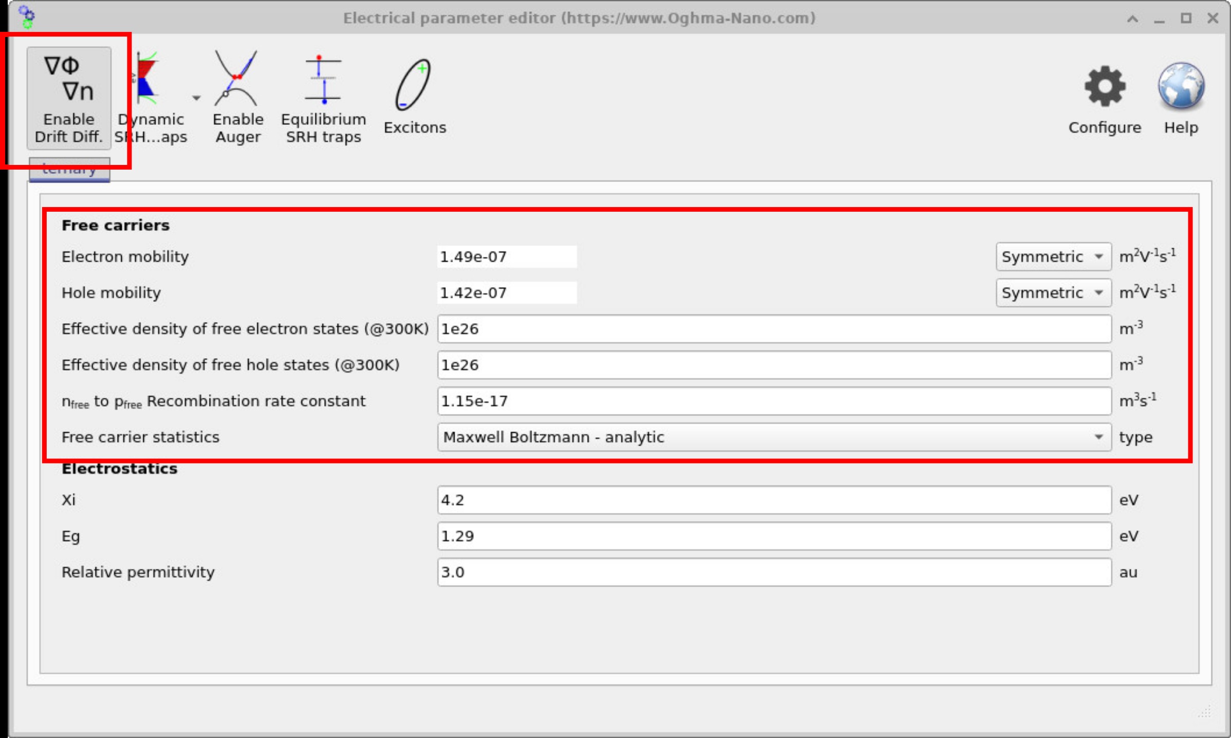
In contrast, Figure ?? shows the same editor with the Enable Drift Diffusion button depressed. When activated, the drift–diffusion solver is enabled and a wider set of parameters becomes available. These include the electron mobility, hole mobility, effective densities of states, and the free-to-free recombination rate constant. Users can also select the form of the free carrier statistics, e.g. Maxwell–Boltzmann or Fermi–Dirac, depending on the material system.

3. Equilibrium SRH traps

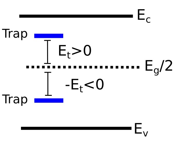
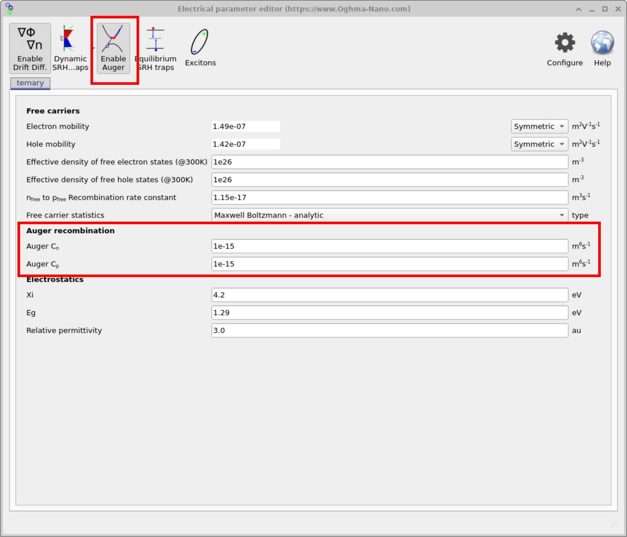
Figure ?? shows the Electrical parameter editor with the relevant recombination controls visible. Enabling Equilibrium SRH traps activates input fields for specifying parameters of a single equilibrium defect level used in the steady-state Shockley–Read–Hall (SRH) recombination model.

In this formulation, recombination is mediated by a single trap level with energy \(E_t\) relative to the middle of the bandgap, a trap density \(N_t\), and electron and hole capture cross-sections \(\sigma_n\) and \(\sigma_p\). These parameters are assumed to describe a population of identical defects that can capture both electrons and holes.

\[ R_{\mathrm{SRH}} = \frac{np - n_{\mathrm{eq}} p_{\mathrm{eq}}} {\tau_p (n + n_1) + \tau_n (p + p_1)} \]

Here \(n\) and \(p\) are the local electron and hole densities, while \(n_{\mathrm{eq}}\) and \(p_{\mathrm{eq}}\) denote their equilibrium values. Writing the numerator in this form guarantees that the net recombination rate vanishes exactly at equilibrium.

The effective carrier lifetimes \(\tau_n\) and \(\tau_p\) are derived from the trap density and capture cross-sections as

\[ \tau_n = \frac{1}{\sigma_n v_{\mathrm{th}} N_t}, \qquad \tau_p = \frac{1}{\sigma_p v_{\mathrm{th}} N_t}, \]

where \(v_{\mathrm{th}}\) is the thermal velocity. The auxiliary SRH quantities \(n_1\) and \(p_1\) are defined in terms of the trap energy relative to the mid-gap reference:

\[ n_1 = n_i \exp\!\left(\frac{E_t - E_{\mathrm{ref}}}{kT}\right), \qquad p_1 = n_i \exp\!\left(\frac{E_{\mathrm{ref}} - E_t}{kT}\right), \]

with \(E_{\mathrm{ref}} = E_g/2\) and \(n_i = \sqrt{n_{\mathrm{eq}} p_{\mathrm{eq}}}\). A trap energy of \(E_t = 0\) therefore corresponds to a mid-gap defect, while positive and negative values shift the trap towards the conduction or valence band, respectively.

Figure ?? illustrates the definition of the trap energy relative to the mid-gap reference. In this simplified equilibrium SRH model, only a single defect level is considered. The sign of \(E_t\) determines whether the trap lies closer to the conduction band (\(E_t > 0\)) or closer to the valence band (\(E_t < 0\)). More general descriptions involving multiple trap levels and explicit capture–emission dynamics are discussed in the dynamic trapping model.

This implementation corresponds to the classical equilibrium SRH model. It does not include explicit trapping and emission dynamics, which are handled separately under the dynamic SRH traps option.

4. Auger recombination

Figure ?? shows the Electrical parameter editor with the Enable Auger button depressed. This activates the Auger coefficient fields \(C_n\) and \(C_p\) (units: \(\mathrm{m^6\,s^{-1}}\)), which parameterise three-carrier recombination under high injection / high carrier density.

\[ R_{\mathrm{Auger}} = \left(C_n\,n + C_p\,p\right)\left(np - n_{\mathrm{eq}}p_{\mathrm{eq}}\right) \]

Here \(n\) and \(p\) are the local electron and hole densities, and \(n_{\mathrm{eq}}\) and \(p_{\mathrm{eq}}\) are their equilibrium values. Writing the driving term as \(\left(np - n_{\mathrm{eq}}p_{\mathrm{eq}}\right)\) ensures the net Auger recombination rate vanishes at equilibrium. Because the prefactor scales with carrier density, Auger recombination is primarily used to capture high-density losses (for example in heavily doped regions or under strong injection).

6. More Complex Distributions of States

By default, the dynamic Shockley–Read–Hall (SRH) model assumes an exponential distribution of trap states. However, experimental studies have shown that the density of states (DoS) in disordered semiconductors is often not purely exponential. In some reports, the distribution is closer to Gaussian; in others, it is best described as a mixture of Gaussian and exponential components; and in more complex cases, entirely different functional forms are required. In all situations, the exact shape of the DoS is strongly dependent on the energetic position of the states within the bandgap.

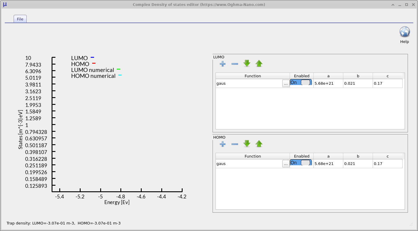
Figure 8 shows the electrical parameters available for defining the DoS of a Shockley–Read–Hall trap distribution. If the DoS type is switched from Exponential to Complex and the Edit button is clicked, the interface shown in Figure ?? appears. Here, users can define arbitrary energetic distributions of trap states, including Gaussian, exponential, Lorentzian, or combinations of these functions.