Shape database
The Shape database acts as a general-purpose local repository of 3D CAD models. Entries in the Shape database are stored as 3D meshes (or shapes) and mayrepresent, for example, the rough surface of a material obtained from AFM measurements, the complex hexagonal contact on a large-area device (see ??), or the periodic pillars of a photonic crystal. Shapes are defined using triangular meshes. The Shape Database window includes tools for generating new 3D CAD models from 2D images, as well as importing external meshes from Wavefront OBJ files. Crucially, all shapes in this database are stored persistently on disk and are intended for representing more complex geometries than those generated by the Mesh editor, which focuses on simple geometric primitives such as boxes, tubes, and spheres (see CAD Meshes).
Accessing the database
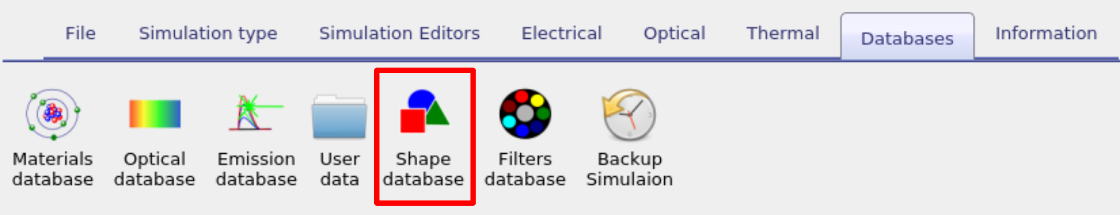
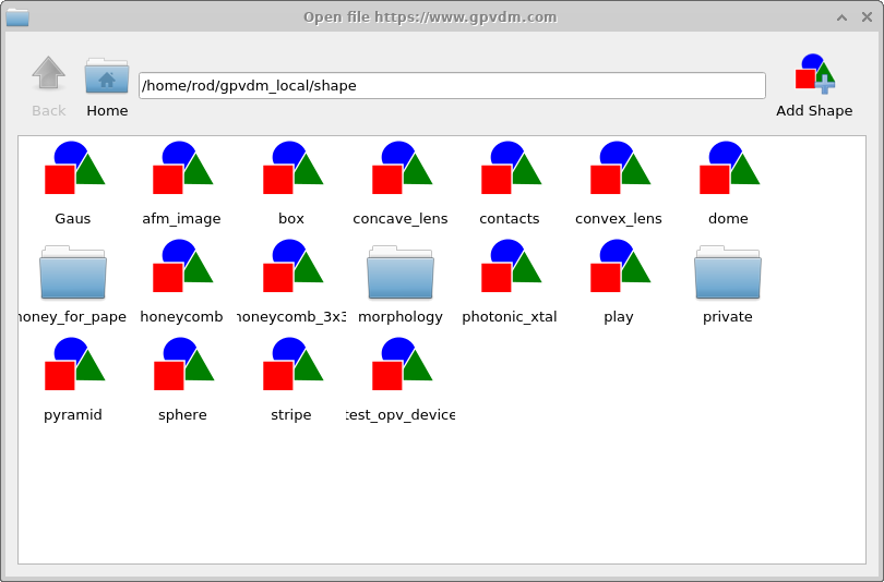
Shapes are stored in the Shape Database, which can be accessed via the Database ribbon by clicking on the Shapes icon (see ??). Clicking the Shape database icon opens the Shape Database window (??).
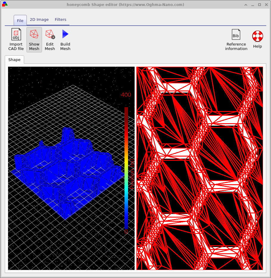
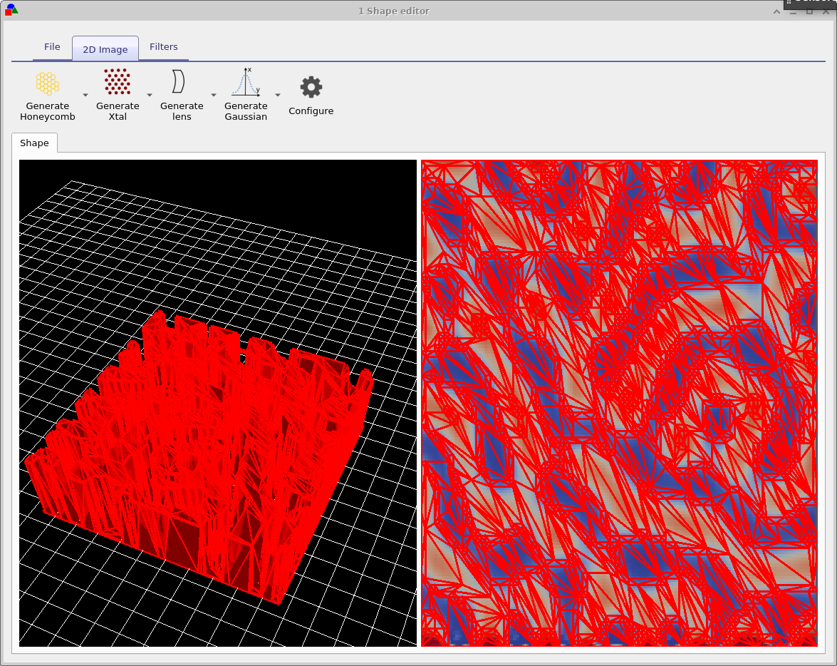
Try opening some of the shapes to inspect them. You will see a window like that in ??. This example shows a honeycomb contact structure of a solar cell. On the left is the 3D shape, and on the right is the 2D image used to generate it. Overlaid on the 2D image is a zx projection of the 3D mesh. You can turn this 2D mesh off and on by toggling the show mesh button in the top ribbon.
Generating a mesh
Once the Shape Database window is open, you can view and edit any stored shape. Many shapes in the database were
originally created from 2D images using the built-in discretisation tools. This section explains how that process
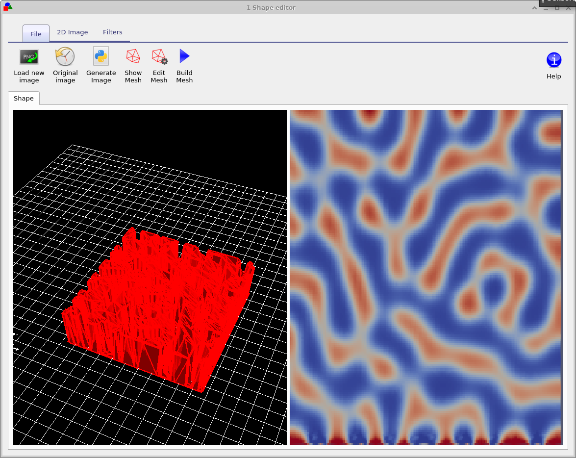
works. Open morphology/1 in the Shape Database. You will see a window similar to
??.
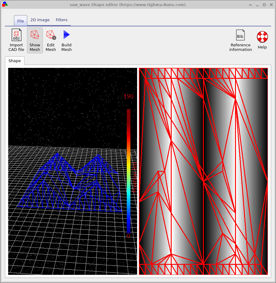
The left panel shows the resulting 3D triangulated mesh, while the right panel displays the original 2D image from
which the mesh was generated. The Show mesh button in the File ribbon toggles the
mesh overlay on the 2D image, letting you inspect how the triangulation follows the underlying features.
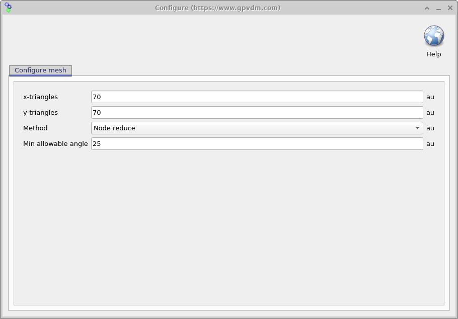
To change how the image is converted into a 3D mesh, click Edit mesh in the File ribbon. This opens the mesh configuration dialog (??), which allows you to control the level of discretisation.
The key parameters are:
- x-triangles — maximum number of triangles along the horizontal direction
- y-triangles — maximum number of triangles along the vertical direction
- Method — selects how the mesh is constructed
- Min allowable angle — prevents extremely thin, unstable triangles
As an example, reduce both x-triangles and y-triangles to 40, then
click Build mesh. The resulting mesh will contain fewer triangles and therefore be less detailed,
but faster to work with. This reduction is visible immediately in the 2D and 3D previews.
The Method setting controls how triangles are generated:
- No reduce: produces a uniform, regular triangular grid. This gives the most accurate geometry but creates a large number of triangles.
- Node reduce: starts from a regular grid and then removes unnecessary points to reduce triangle count while preserving the overall shape.
Switching to No reduce and rebuilding the mesh will replace the adaptive mesh with a full, regular 70 × 70 triangulation. This is more precise, but also heavier to store and simulate. Every additional triangle in a mesh introduces extra computational burden in a simulation. The goal when building a mesh is therefore to represent the shape using as few triangles as possible. If you can describe an entire surface with a relatively small number of triangles, it is usually worth doing so. For very regular shapes, however, applying Node reduce to cut down the triangle count may offer little or no benefit; in such cases a simple regular mesh can be just as effective. In practice, you will often need to experiment with different settings and methods to find a mesh that gives an acceptable balance between accuracy
and computational cost.
2D image generation and filtering tools
In addition to loading images from file, the Shape Editor contains a set of tools for generating new 2D patterns that can be converted into 3D meshes. These tools are located under the 2D Image ribbon and include generators for a wide range of structures:
- Honeycomb patterns for pixel layouts or electrode grids
- Photonic crystal lattices with configurable periodicity
- Lenses defined as height maps
- Gaussian profiles for bumps, pits, or graded surfaces
- Saw-wave height functions (example shown below)
- Checkerboard patterns for calibration and testing
- Perlin noise for generating realistic surface roughness
Each generator provides its own configuration options, allowing you to customise the geometry before converting it into a mesh. These images act as height maps or masks, from which the Shape Editor constructs the corresponding 3D structure.

After generating or loading an image, the Filters ribbon provides tools for modifying it before mesh construction. These include:
- Blur — smooths noise or sharp transitions
- Normalize (x, y, z) — rescales the image in each direction
- Threshold — converts the image to a binary mask (example shown above)
- Rotate — rotates the pattern by fixed or arbitrary angles
- Boundary — emphasises or extracts boundaries within the image
These tools allow you to refine height maps, clean noisy images, or manipulate patterns prior to generating the final triangular mesh. The combination of image generators and filters provides a flexible workflow for creating complex, custom 3D geometries directly inside OghmaNano.
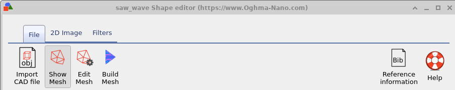
Importing from CAD files
In addition to generating shapes from 2D images, the Shape Editor also allows you to import external 3D meshes using the Import CAD file button shown in ??. OghmaNano supports the Wavefront OBJ format, which is widely used for storing triangulated surface meshes. You will also find in the Shape Database an example of an imported CAD model: the classical Utah Teapot, shown in ??. This mesh illustrates how external triangulated models appear once imported into the editor.
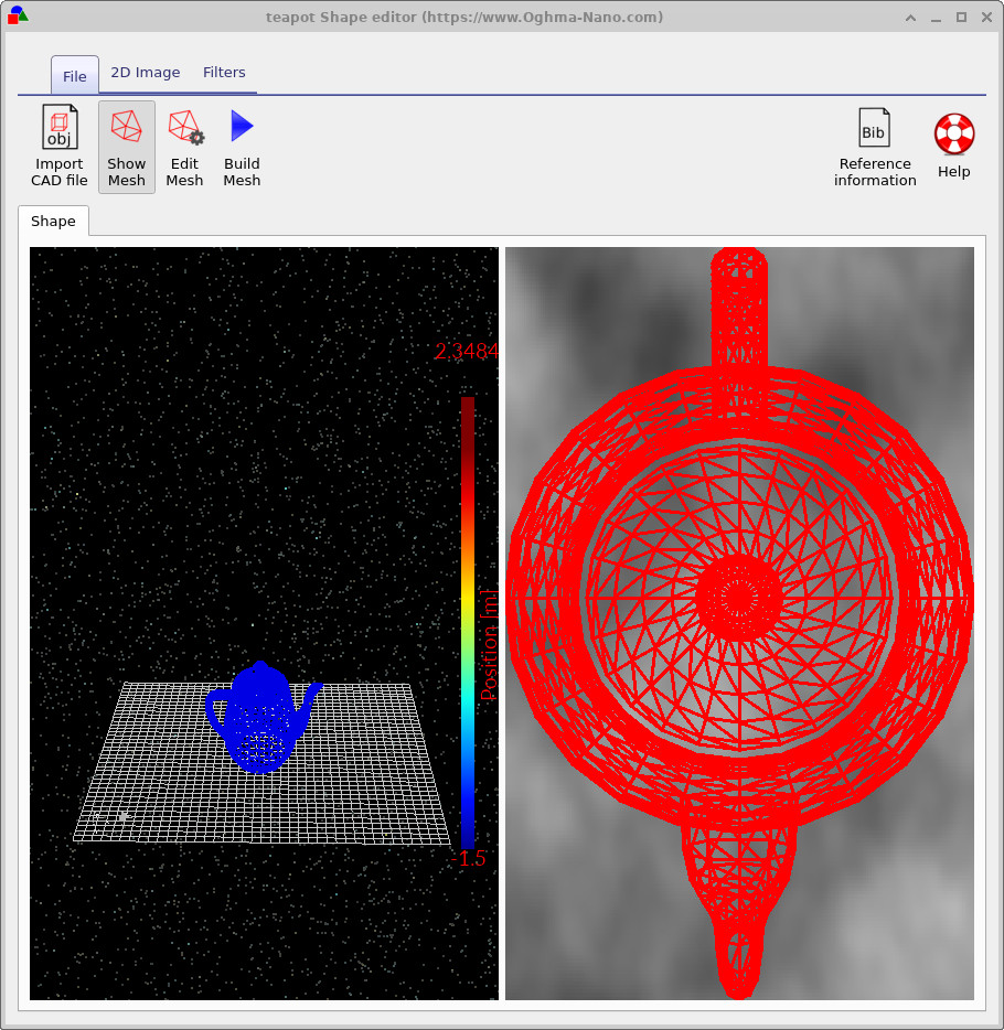
When importing CAD models, it is important to ensure that the mesh forms a closed surface. A closed surface is one in which every edge belongs to exactly two triangles, producing a completely sealed, watertight volume. Open surfaces, missing faces or cracks lead to ambiguity in determining whether points lie inside or outside the object, which makes them unsuitable for simulation.
CAD meshes are typically designed for machining and manufacturing, not numerical simulation. As a result, they often contain far more triangles than necessary for optical or physical modelling. A large triangle count significantly increases computation time in ray tracing and other solvers.
For best performance, ensure that imported meshes:
- form a fully closed, watertight surface,
- contain only as many triangles as needed to represent the geometry, and
- have unnecessary fine features or machining artefacts removed.
Following these guidelines will help ensure that imported CAD geometries run efficiently within OghmaNano.
The shape file format
A shape must form a fully enclosed volume. If you use the built-in shape discretiser this condition is enforced automatically. However, if you construct shapes by hand you must ensure that the volume is closed.
Each shape directory contains the following files:
| File name | Description | |
|---|---|---|
| \(data.json\) | Configuration data for the shape. | |
| \(image\_original.png\) | Backup of the imported image. | |
| \(image\_out.png\) | The final processed image. | |
| \(image.png\) | The working copy of the imported image. | |
| \(shape.inp\) | The discretised 3D mesh of the shape. |
The PNG files represent the image in different stages of processing. The data.json file stores the
configuration of the Shape Editor, and the shape.inp file contains the 3D structure of the object.
An example shape.inp file is shown in
??.
The format is designed so that gnuplot can open it directly using the splot command.
Each triangle is described by four z, x, y points: the first three lines define the triangle, and the
fourth repeats the first point so that gnuplot can plot a closed outline. The number of triangles in
the file is defined on a line beginning with #y.
The exact magnitudes of the z, x, y values do not matter. As soon as the shape is loaded, all values
are normalised so that the minimum point of the shape sits at (0, 0, 0) and the maximum point lies at
(1, 1, 1). When the shape is inserted into a scene, it is renormalised to the desired physical size
of the object in the device.
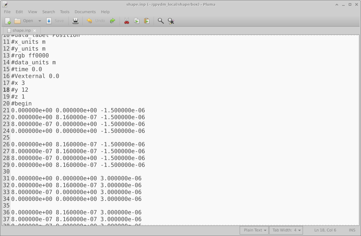
shape.inp file. Each triangle is defined by four z, x, y points and can be
visualised directly using gnuplot.
👉 Next step: For a worked example of how to generate shapes, please see the tutorial on the Shape Database and how to create 3D shapes from images at this link.