Fabry-Pérot Cavity Simulation Using the Transfer Matrix Method (TMM)

1. Introduction

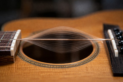
A Fabry-Pérot cavity is a resonant optical structure formed when light is confined between two partially reflecting boundaries. Multiple reflections inside the cavity cause the optical waves to interfere with one another, producing standing-wave resonances at specific wavelengths. Wavelengths satisfying the cavity resonance condition experience enhanced transmission and strong optical field buildup inside the structure.

Fabry-Pérot resonators are widely used in optical filters, dielectric mirrors, interferometers, LEDs, and laser cavities. In this tutorial, we model a simple one-dimensional Fabry-Pérot cavity using the transfer matrix method (TMM).

Unlike FDTD, which numerically propagates the electromagnetic field through both space and time, the transfer matrix method assumes a one-dimensional layered structure and solves for the optical fields analytically within each layer. The electromagnetic field is represented as a superposition of forward and backward travelling waves, with the fields connected across interfaces using Maxwell boundary conditions. For planar multilayer systems, this greatly reduces the computational complexity, making TMM extremely efficient for analysing cavity resonances and thin-film interference effects. A full derivation of the transfer matrix method is given in Transfer matrix theory.

At normal incidence, the Fabry-Pérot resonance condition is

\(2nL = m\lambda\)

where \(n\) is the refractive index inside the cavity, \(L\) is the cavity length, \(\lambda\) is the wavelength, and \(m\) is an integer mode number.

Rearranging gives the allowed cavity wavelengths:

\(\lambda_m = \frac{2nL}{m}\)

This means that only discrete resonant wavelengths are efficiently transmitted through the cavity. In this tutorial, we will directly observe these resonances in the transmission and reflection spectra, and also visualise the standing-wave photon density inside the cavity.

2. Making a new simulation

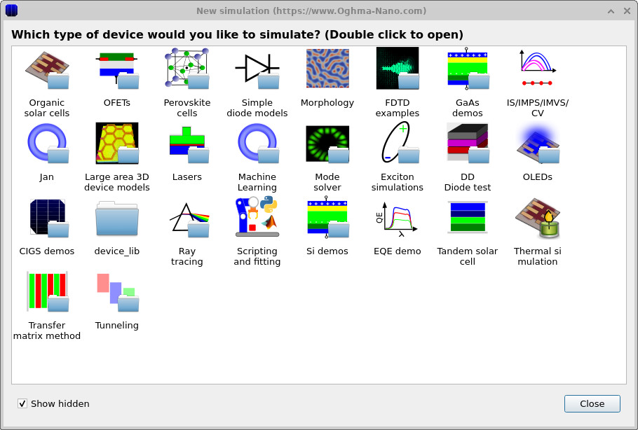
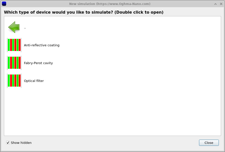
Open the New simulation window and select the Transfer matrix method category (??). Then select the Fabry-Pérot cavity example (??).

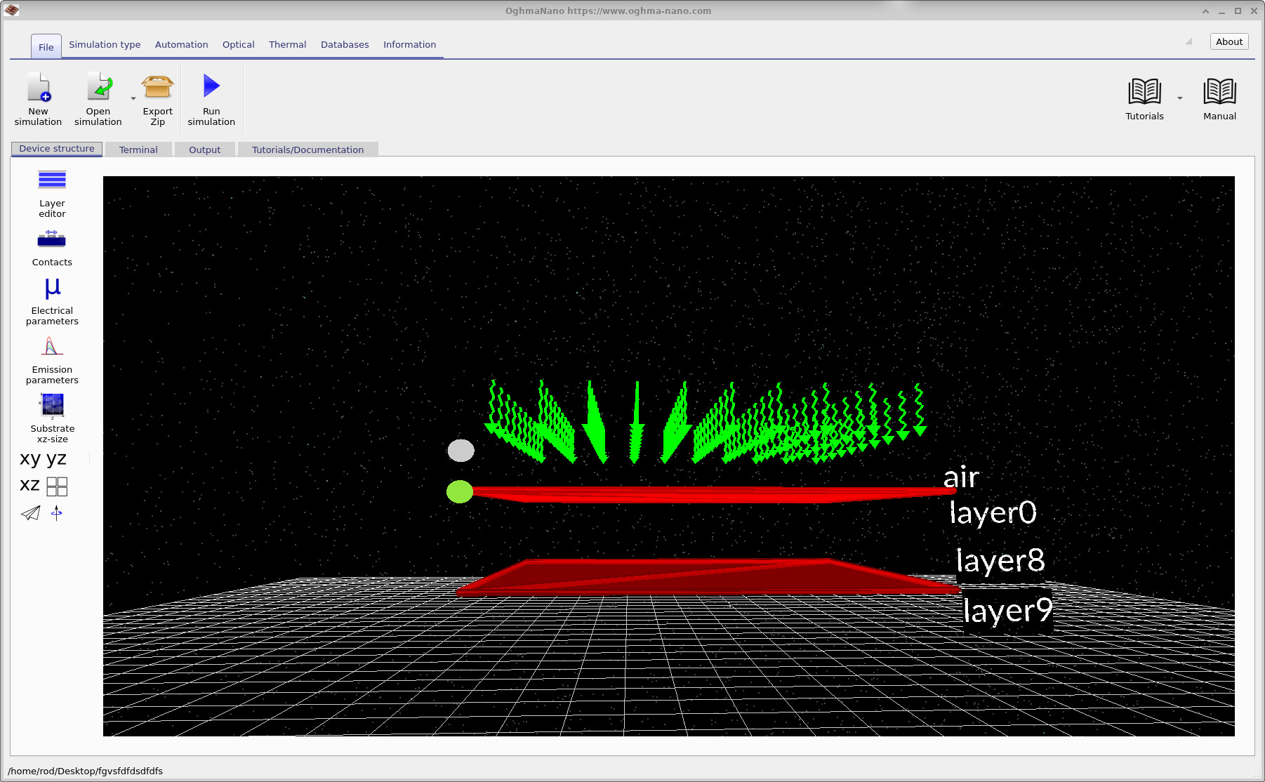
After opening the example, the main interface appears as shown in ??. The simulation consists of a simple optical cavity formed by two partially reflecting layers separated by an air gap.

The cavity consists of two thin dielectric layers with refractive index \(n=3\), separated by an air region. These two high-index layers act as partially reflecting mirrors.

When broadband light enters the structure, multiple reflections occur between the mirrors. At wavelengths satisfying the cavity resonance condition, the reflected waves interfere constructively, producing enhanced field buildup inside the cavity and increased transmission through the structure.

3. Running the optical simulation

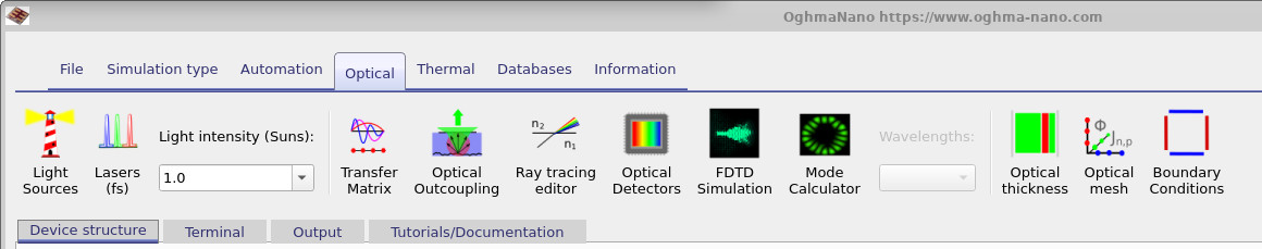
Open the Optical ribbon (??) and click the Transfer Matrix button. This launches the optical transfer matrix solver.

The transfer matrix method computes the optical field distribution, reflection spectrum, transmission spectrum, and absorbed photon density throughout the multilayer structure. Because this method works directly in the frequency domain, simulations typically complete in only a few seconds.

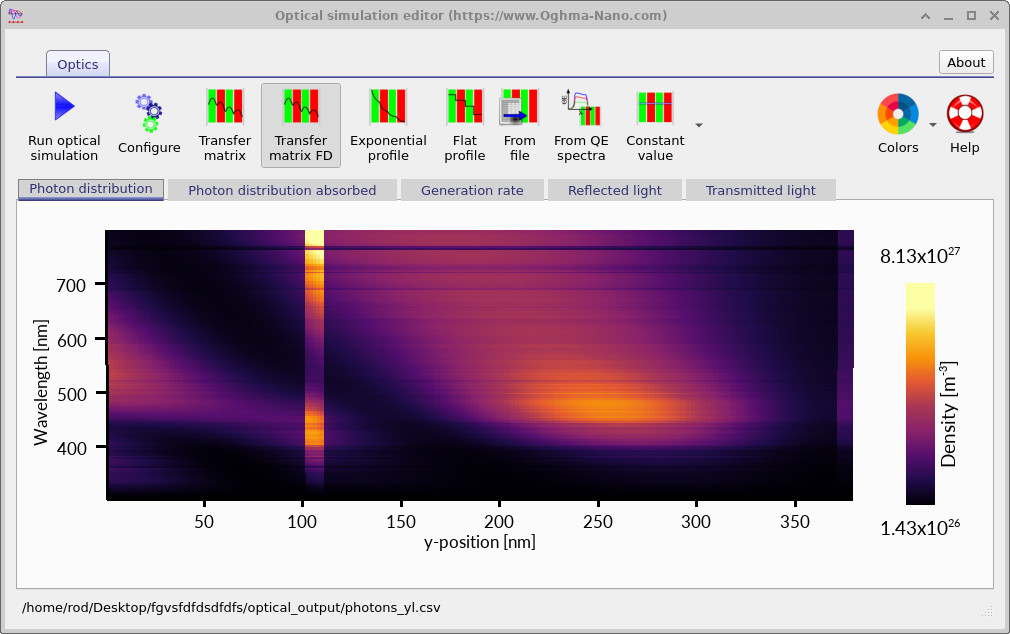
After the simulation finishes, the photon-density map shown in ?? appears. The horizontal axis corresponds to position inside the cavity, while the vertical axis corresponds to wavelength.

Bright regions indicate wavelengths where the optical field builds up strongly inside the structure. The most prominent feature occurs near 450-500 nm, corresponding to the fundamental Fabry-Pérot resonance of the cavity.

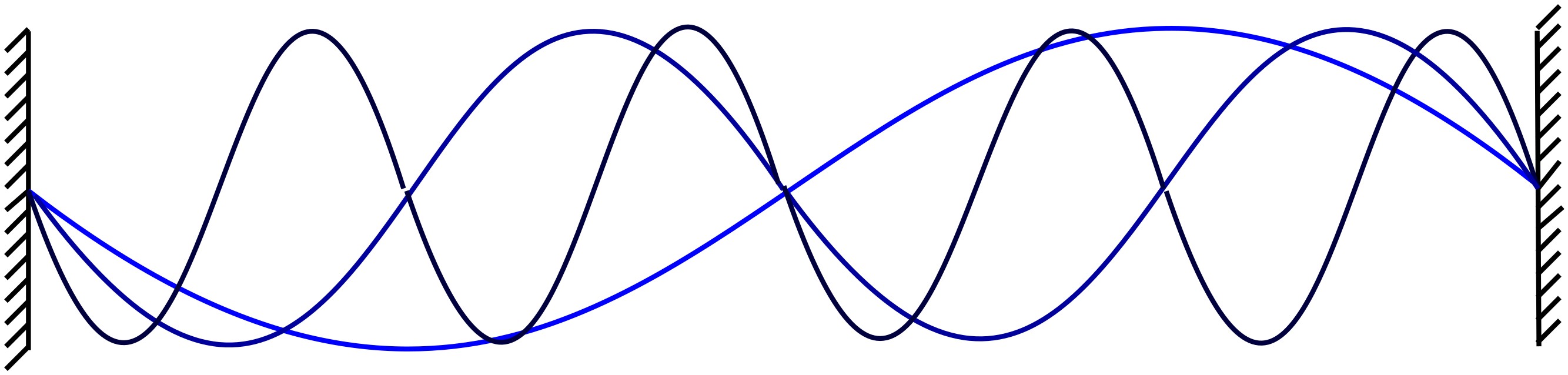
The oscillatory spatial structure visible in the plot is the standing-wave pattern formed by interference between forward and backward travelling waves inside the cavity.

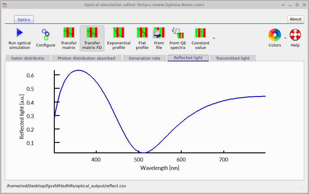
4. Reflection and transmission spectra

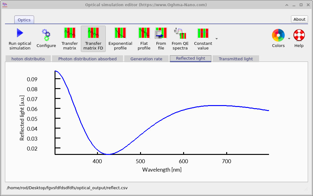
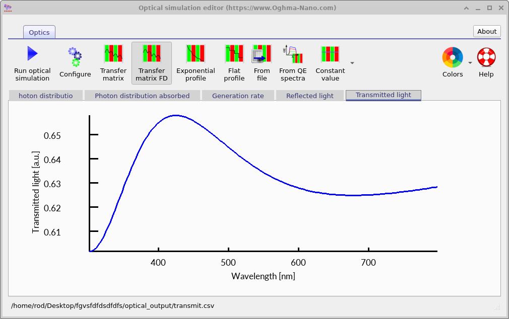
The transfer matrix solver also calculates the reflected and transmitted optical power. These results are shown in ?? and ??.

The cavity resonance appears as a pronounced dip in the reflection spectrum and a corresponding peak in the transmission spectrum. Physically, this occurs because the cavity stores optical energy efficiently at the resonant wavelength, allowing light to pass through the structure rather than being reflected.

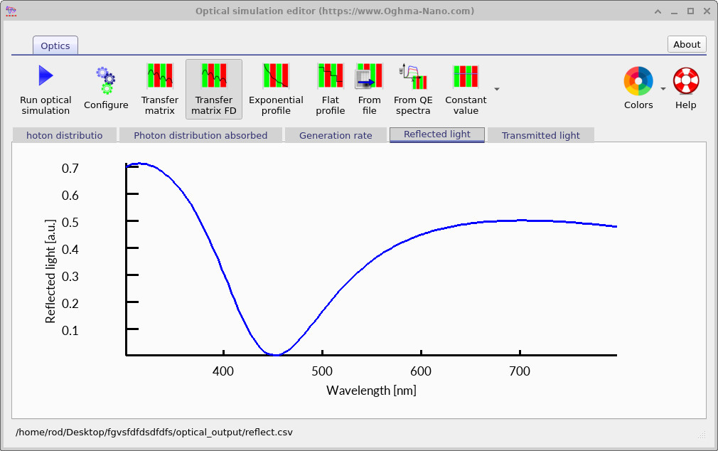
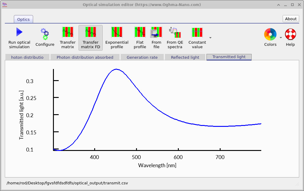
In this structure, the cavity spacing is approximately 250 nm and the cavity refractive index is close to 1. The resonance condition therefore predicts a fundamental mode near

\(\lambda \approx 2nL \approx 2 \times 1 \times 250 \approx 500\ \text{nm}\)

which is consistent with the spectra observed above.

5. Changing the cavity length

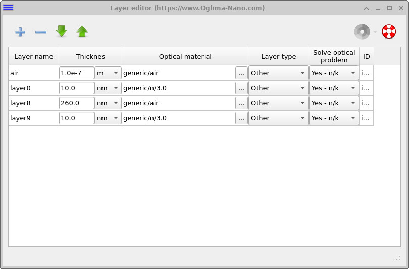
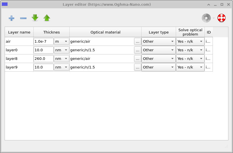
Open the Layer editor shown in ??. The cavity is formed by two thin dielectric layers separated by an air gap.

In the original structure, the cavity thickness is approximately 260 nm. Increase this to 300 nm, as shown in ??, then rerun the optical simulation.

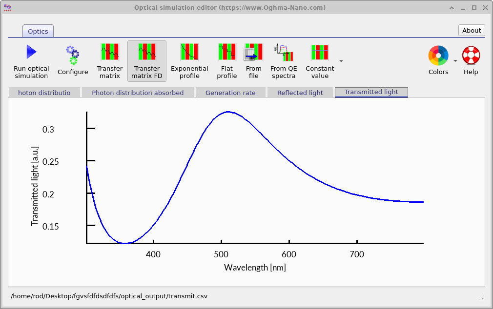
After rerunning the simulation, the spectra shown in ?? and ?? are obtained.

Increasing the cavity length shifts the resonance toward longer wavelengths. This follows directly from the Fabry-Pérot condition:

\(\lambda = \frac{2nL}{m}\)

Since the resonance wavelength is proportional to cavity length, increasing \(L\) causes the transmission peak to move systematically toward larger wavelengths.

You should also observe additional weaker resonances corresponding to higher-order cavity modes (\(m=2,3,\dots\)).

6. Viewing photon-density snapshots

Return to the Output tab shown in ??. Open the optical_snapshots directory to inspect the photon-density distribution at individual wavelengths.

The snapshot viewer allows the optical field distribution to be examined at specific wavelengths throughout the cavity structure. Unlike the wavelength-position maps shown earlier, these snapshots provide a direct view of the standing-wave pattern formed inside the cavity at a single wavelength.

Example photon-density distributions are shown in ??- ??.

These plots show the spatial photon-density distribution inside the Fabry-Pérot cavity. The oscillatory behaviour arises from interference between forward and backward travelling optical waves reflected by the two cavity mirrors. Regions of high photon density correspond to standing-wave antinodes, while minima correspond approximately to standing-wave nodes.

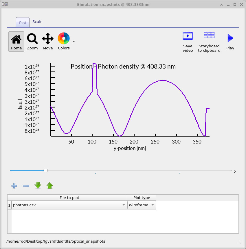
The photon-density snapshots shown in ??- ?? provide a direct view of how light behaves inside the Fabry-Pérot cavity. Rather than simply passing through the structure once, the optical wave repeatedly reflects between the two partially reflecting mirrors. These multiple reflections interfere with one another and form standing-wave patterns inside the cavity.

The alternating peaks and valleys visible in the photon-density distributions correspond to the standing-wave structure of the optical field. Regions of high photon density are standing-wave antinodes, where the electric field oscillation is large, while the minima correspond approximately to standing-wave nodes, where destructive interference suppresses the field.

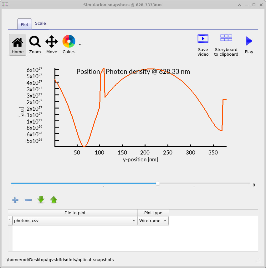
In ??, the standing-wave pattern is strongly concentrated near the left-hand side of the cavity. The narrow high-intensity feature near the interface indicates that the optical field is being strongly reflected and confined close to the mirror. Moving across the cavity, the field oscillates and gradually redistributes throughout the structure. In ??, the optical field becomes much more evenly distributed across the cavity region. At this wavelength the cavity is closer to a resonant condition, allowing the reflected waves to reinforce one another more efficiently. Instead of being concentrated near a single interface, the optical energy builds up throughout the cavity, producing the broad standing-wave pattern visible in the figure.

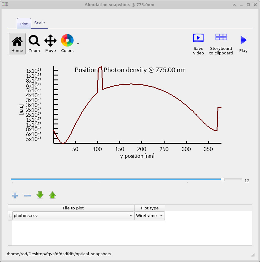
In ??, the standing-wave spacing becomes larger because the optical wavelength inside the cavity has increased. The field extends smoothly across almost the entire cavity, while still showing the characteristic oscillatory behaviour produced by interference between forward and backward travelling waves. The abrupt vertical transitions visible near the cavity interfaces arise from changes in refractive index between adjacent layers. At these boundaries the electromagnetic field must satisfy Maxwell boundary conditions, causing the amplitudes of the forward and backward travelling waves to adjust suddenly at the interfaces.

These figures illustrate one of the key physical ideas behind Fabry-Pérot cavities: the cavity only stores light efficiently at certain wavelengths. When the optical phase condition is satisfied, the reflected waves reinforce one another and a stable standing-wave mode forms inside the structure. At non-resonant wavelengths this constructive interference does not occur, so the optical field buildup becomes much weaker and more of the incident light is reflected away from the cavity.

7. Changing the refractive index contrast

The strength of the cavity resonance depends strongly on the reflectivity of the mirrors. In dielectric Fabry-Pérot cavities, this reflectivity is controlled primarily by the refractive-index contrast.

Open the layer editor and reduce the mirror refractive index from \(n=3\) to \(n=1.5\), as shown in ??.

After rerunning the simulation, the reflection and transmission spectra become those shown in ?? and ??.

When the refractive-index contrast is reduced, the mirrors become weaker reflectors. This reduces the amount of light trapped inside the cavity and broadens the resonant features.

Physically, this corresponds to a reduction in cavity quality factor (Q-factor). Strong mirrors produce narrow resonances with strong field buildup, while weak mirrors produce broader and less pronounced resonances.